DPE

• 
• 

The DPE (Data Processing Engine) is a software tool which serves for a processing of data acquired with the Timepix detectors (TPX, TPX2, TPX3). The following list includes the main processing parts of the DPE:

• Pre-processing: clustering of data with application of calibration and corrections, calculation of cluster variables/parameters, creation of histograms
• Processing: particle recognition and radiation field recognition
• Post-processing: directional analysis, coincidence analysis, Compton camera, generation of physical products and their time evolution with respect to the radiation field classification (fluxes, dose rates etc.)

Following information is valid for version 1.1.0.

• 

  Example of particle classification for data acquired onn board of ISS with TPX3 500um.

• 
• 
• 
• 
• Error creating thumbnail: File with dimensions greater than 12.5 MP

Download

The data processing engine can be downloaded from the following sources based on the needed computer configuration:

Operataion system	Link
Linux	Media:DPE_1_1_0_Linux.zip
Windows x64	Media:DPE_1_1_0.zip

The linux version was built on Ubuntu 20.04 with g++ version 9.4.0.

Following links can be used to download API in C++:

Operataion system	Link
Linux API c++	Media:DPEApiCpp_1_1_0_Linux.zip
Windows API c++	Media:DPEApiCpp_1_1_0.zip

Examples of DPE usage for sevetal cases can be downloaded from the following link:

File	Link
Examples	Media:DPE_Example.zip

Prerequisites, Install and Run

In the directory, where it should be “installed”, download and extract all files of OS directories (Linux or Windows). The ParametersFile.txt includes settings of the program/engine, see description in the next section. There are several other configuration files which set other processing parts of DPE (histograms, filters, masking etc.) and they are also described in individual sections of this document.

To create graphics, python3 and several packages are needed:

• matplotlib (version >= 3.4)
• numpy
• multiprocessing - only if creation of graphics should be done on several threads/cores of CPU

The program, especially in the case of graphic export, needs several hundreds of MB on RAM (app 500 MB but it is based on the size of exported histograms). If the multiprocessing is used then the RAM usage can be up several GB and all threads of the CPU might be used.

Run the program on linux

     ./dpe.sh  PARAMETERS_FILE_PATH/PARATERS_FILE_NAME

PARAMETERS_FILE_PATH is path to the parameters file and PARATERS_FILE_NAME is its name. It is possible that dpe.sh and clusterer have to be allowed as an executable: chmod +x clusterer.

Run the program on windows

    DPE.exe PARAMETERS_FILE_PATH\PARATERS_FILE_NAME

If your path or name of the parameters includes white spaces enclose it in quotes: “PARAMETERS_F ILE_ PATH_F ILE_NAME”. The input parameter into the DPE containing the path and name of the parameter file can be omitted if the file is in the same directory as the DPE and its name is ParametersFile.txt.

First Example of Run

This sections includes information about the first run of the DPE based on the ParamteresFile given with the program example. Example directory can be found and downloaded for the same download link. It includes needed inputs for the example to run on linux and windows systems. In the case of running example on linux system then it is needed to download following directories: Linux, Clusterer, Example. The example can be run with following command from the Linux directory:

    chmod +x dpe.sh
    ./dpe.sh ./ParametersFile.txt

The output should be exported into the Example/Output directory. The given data is a mixed sample of proton, electron and alpha ion data measured with TPX3 500 um. Run of the DPE should read the main parameters file ParametersFile.txt and create several export directories with files and graphics:

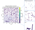
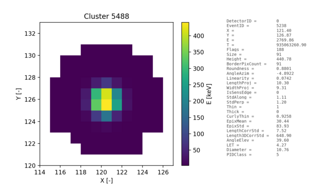
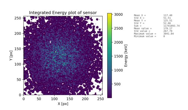
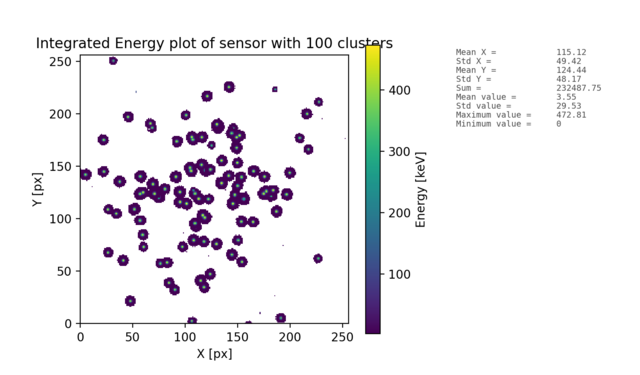
• EventVisual - individual cluster plots, integrated sensor plots and plots of clusters for individual PID classes.
• File - main data files: elist, cluster log and sampling list.
• Graph - graphical representation of the sampling list.
• Hist - histograms of cluster variables.
• SpatialMap - spatial maps of cluster variables also with respect to the PID classes.
• SigVec - significant vector which uniquely specifies the given radiation field.
• Direction - results of directional analysis: estimation of radiation direction.
• CoincEvent - results of coincidence analysis: evaluates time correlation between clusters.

The main configuration is done in the ParametersFile.txt and meaning of individual parameters can be found directly there or in this document. Other files in the Example directory determine the creation of histograms (Hist.ini), masking of the raw data (Mask.txt), filtering of cluster (Filter.ini) and creation of the SigVec (SigVec.ini). Pre-generated referential results can be found in the directory Ref. More information about their format can be found in the next sections in this document.

The similar example can be also made on Windows with alternative command from the directory Windows:

    DPE.exe .\ParametersFile.txt

The output and its description is the same as the for the linux system above.

Additional Examples

Additional examples can be found in the directory Example/Test which includes several examples from testing. The input data are in directory data and its output can be found in the directory ref (referential output). The examples comprehend following cases:

1. T3PA input - t3pa input with default settings (Am241 source).
   
2. Several T3PAs input - 20x t3pa files as input with default settings (Am241 source).
   
3. CLOG tot+toa TPX3 input - clog tot+toa from TPX3 with default settings (Am241 source).
   
4. CLOG tot TPX input - clog tot from TPX with default settings (protons HE).
   
5. CLOG itot+count TPX3 input - clog itot+count from TPX3 with default settings (Am241 source).
   
6. Hist with T3PA - Hist settings with T3PA file as input.
   
7. Filter with T3PA - Filter settings with T3PA file as input (Am241 source).
   
8. SigVec with T3PA - SigVec settings with T3PA file as input
   
9. Mask with T3PA - Mask settings (general file) with T3PA file as input
   
10. Comparator with T3PA and CdTe - Comparator with T3PA file as input
    
11. Elist old input - elist as input with default settings
    
12. Generated t3pa input - pregenerated t3pa for physical variables etc.
    
13. SigVec and Hist with T3PA - SigVec and Hist settings with T3PA file as input to produce SigVec from 2D hist.
    
14. CLOG event input - clog event with default settings.
    
15. CLOG toa input - clog toa with default settings.
    
16. CLOG tot+time proc input - clog tot+time after processing with default settings.
    
17. T3P input - t3p input with default setting (ba133)
    
18. T3R input - t3r input with default settings (upper part of detector was masked)
    
19. Matrix event input - matrix event input with default settings
    
20. Matrix tot input - matrix tot input with default settings
    
21. Elist extended input - elist extended input with default settings
    
22. Graphics output CLOG tot+toa TPX3 input - graphics output for CLOG tot+toa TPX3 input with default settings
    
23. Several T3PAs input, just dir name - several t3pa files, just specifying dir name as input with default settings
    
24. Comparator with own DB - input is own DB for camparator and settings of SigVec and Hist for t3pa input
    
25. Print program version - print program version with -v
    
26. Print program help - print program help with -h
    
27. Ignore clusters at sensor edge - remove clusters at sensor edge with default settings with T3PA file as input
    
28. Pixet mask with T3PA - Mask settings (pixet mask) with T3PA file as input
    
29. Acceptance of all param - param file with all params and their acceptanc.
    
30. CLOG tot+toa meas input - clog tot+toa from measurement with default settings
    
31. Generated t3pa 2x - pregenerated t3pa two times to check connection of two separate measurement files
    
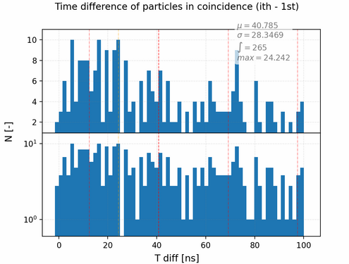
32. Coincidence analysis - coincidence and matching analysis (time coincidence window and products)
    
33. Directional analysis - directional analysis with proton 200 MeV 75 deg data.
    
34. Compton analysis single forward - Compton analysis for single layer forward (other analysis are off due to pregenerated data).
    
35. Compton analysis single forward - Compton analysis for single layer forward (other analysis are off due to pregenerated data).
    
36. RadFiledRecog analysis - radiation field recognition for 2mm CdTe TPX3 with Ba133 data.
    
37. RadFiledRecog analysis - radiation field recognition for 2mm CdTe TPX3 with Cs137 data.
    
38. Frame analysis - frame analysis.
    
39. Detector geometry - setting of geometry via geo det config file.
    
40. Adv elist - advanced elist.
    
41. Adv elist extended - advanced elist extended in dpe.
    
42. All analysis and their switches - using all analysis and turning them off compatibility.
    
43. Length correction option - setting different length correction.
    
44. High energy correction TPX - using high energy correction for TPX alpha Am241 (200V, peak around 3 MeV).
    
45. Err - missing param file - error behavior without parameters file
    
46. Err - empty file - error behavior with empty file file
    
47. Err - simple elist - error behavior with simple elist
    
48. Err - nonsense file - error behavior with nonsense file
    
49. Err - empty clog - error behavior with empty clog
    
50. Err - incorrect clog - error behavior with incorrect clog
    
51. Err - partial elist - error behavior with partial elist
    
52. Err - dsc file - error behavior with dsc file
    
53. Err - matrix toa - error behavior with matrix toa
    
54. Err - module configs without path - error behavior of module configs wrong path

All examples were produced on linux system but they should be also valid for windows system.
Note that some of the examples were written with older syntax from previous versions.
This syntax is still valid, but not stated in the list below and it should be easy to follow which names were replaced with the new ones (e.g. CalMatrix_Path to CalMat).

Issues and Help

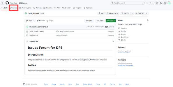
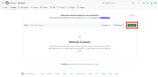
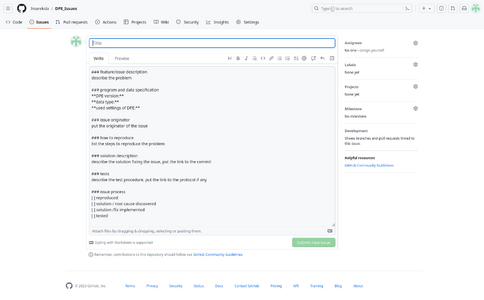
Any ideas or issues can be reported on github forum for issues:

https://github.com/lmareksla/DPE_Issues/

or send directly on the first mail below.

For more information or help: lukas.marek@advacam.cz, carlos.granja@advacam.cz.

• 
• 
• 

Main Configuration of DPE

The main settings of the DPE is done through the so-called parameters file which is a text file with all paths, names and switches to configure the DPE. It has similar notation as the c++ code and example can be found in the directory with the program.
There are several other features of DPE which are handled with different configuration files e.g. filtering, histograms etc. Their settings is mentioned in the next sections.

Syntax of the Parameters File

• Everything which is after // is taken as a comment and the program ignores it (gives opportunity to create comments or easily test different settings).
• Every string should be enclosed in quotes " to correctly account for white spaces in the string. Example: FileName = "file name.txt".
• Number can be written in the common notations, e.g. 2e5, 50, -666.12, .1 (same as 0.1) . Example: Number = 1e7.
• If an array of values is needed then it is separated with comma symbol: , (white spaces are unimportant). Example: ArrayNumbers = 12,13, 14, 15, ArrayString = "hop", "skok"
• The syntax is partially based on the c++ so it can be used in some highlighting text editors for better clarity.
• All used paths are checked for proper slashes of paths which means that same configuration files can be used on windows and linux. This is not valid for the input argument into DPE = path and name of the configuration file.
• It is also possible to convert all parameters to snake case: CalMat to cal_mat (only those which are listed below, it is not compatible with older versions of DPE).

List of Parameters

Name	Type	Description	Example	Default
CalMat	STRING	Path to a directory with calibration matrices if data should be calibrated during pre-processing.	CalMat="/Path/To/Cal/Matrices/"	empty string
ClogOutName	STRING	Name of the cluster log file for export without suffix/ending. If it is stated in the parameters file then the clog is created (alias DoCreateClog = true).	ClogOutName="ClusterLog"	ClusterLog
ClusterCount	INT	Count of clusters which should be processed and evaluated.	ClusterCount=1 ClusterCount=10000 ClusterCount=5
ClusterCountInSensImage	INT	Count of clusters which will be exported in the integrated sensor plots (also per class). It can be less, if there is no such a count of needed clusters set by this value.	ClusterCountInSensImage=10 ClusterCountInSensImage=1000	100
ClustererName	STRING	Name o the clusterer binary. Default, it is decided based on the operation system.	ClustererName="clusterer" ClustererName="clusterer.exe"	clusterer (linux) or clusterer.exe (windows)
ClustererPath	STRING	Path to the clusterer program (part of the download package).	ClustererPath="/Path/To/Clusterer/ Program/"	./Clusterer/
ClusterImageCount	INT	Count of clusters which will be exported as individual cluster plots.	ClusterImageCount=20 ClusterImageCount=1	15
CoincEventListBaseName	STRING	Base name of the coinc_event list which is used for txt and also for the json format. It is combined as this name and adding .txt and .json.	CoincEventListBaseName="CoincEventList" CoincEventListBaseName="List" CoincEventListBaseName="Name"	CoincEventList
CoincEventListJsonName	STRING	Name of output coinc_event list in json format.	CoincEventListJsonName="SampligList.json"	CoincEventList.json
CoincEventListName	STRING	Name of the output coinc_event list.	CoincEventListName="CoincEventList.txt"	CoincEventList.txt
ComptonListBaseName	STRING	Base name of the compton list which is used for txt and also for the json format. It is combined as this name and adding .txt and .json.	ComptonListBaseName="ComptonList" ComptonListBaseName="List" ComptonListBaseName="Name"	ComptonList
ComptonListJsonName	STRING	Name of output compton list in json format.	ComptonListJsonName="SampligList.json"	ComptonList.json
ComptonListName	STRING	Name of the output compton list.	ComptonListName="ComptonList.txt"	ComptonList.txt
ComptonName	STRING	Name of the file with Compton direction reconstruction configuration.	ComptonName="Compton.ini"	empty string
ComptonPath	STRING	Path to the file with Compton direction reconstruction configuration.	ComptonPath="/Path/To/Compton/Config/"	empty string
DetGeoName	STRING	Name of the file with detector geometry configuration.	DetGeoName="DetGeo.ini"	empty string
DetGeoPath	STRING	Path to the file with detector geometry configuration.	DetGeoPath="/Path/To/DetGeo/Config/"	empty string
DirectionListBaseName	STRING	Base name of the direction list which is used for txt and also for the json format. It is combined as this name and adding .txt and .json.	DirectionListBaseName="DirectionList" DirectionListBaseName="List" DirectionListBaseName="Name"	DirectionList
DirectionListJsonName	STRING	Name of output direction list in json format.	DirectionListJsonName="SampligList.json"	DirectionList.json
DirectionListName	STRING	Name of the output direction list.	DirectionListName="DirectionList.txt"	NClusters
DirectionName	STRING	Name of the file with directional analysis configuration.	DirectionName="Direction.ini"	empty string
DirectionPath	STRING	Path to the file with directional analysis configuration.	DirectionPath="/Path/To/Direction/Config/"	empty string
DoClustererLog	BOOL	Export clusterer log. Only valid if clusterer is used during processing (raw data).	DoClustererLog=true DoClustererLog=false	true (used)
DoCompton	BOOL	Control whether Compton directional reconstruction should be done. There is limited list of cases when this analysis is usable based on the detector settings (see section below).	DoCompton=true DoCompton=false	true (if configuration allows)
DoCreateClog	BOOL	Control for a generation of the clog.	DoCreateClog=true DoCreateClog=false	true (used)
DoCreateElistExt	BOOL	Switch to produce elist with additional columns from processing output: filter pass or not passed (1,0), PID class (e.g. from -1 to 8). It is placed as the last columns of the elist with name `FilterPass, PIDClass`.	DoCreateElistExt=FileIn_Count	true (used)
DoDirection	BOOL	Control whether Compton directional reconstruction should be done. There is limited list of cases when this analysis is usable based on the detector settings (see section below).	DoDirection=true DoDirection=false	true
DoDirectionTrackCond	BOOL	Control to use tracking condition during directional analysis (additional constrain on features of clusters).	DoDirectionTrackCond=true DoDirectionTrackCond=false	false
DoDoseUnitRadiology	BOOL	Switch to change from the dose rate in uGy/h to Gy/s.	DoDoseUnitRadiology=true DoDoseUnitRadiology=false	false
DoExportElistExtFilter	BOOL	Control whether clusters which were filtered out should not be exported into extended elist.	DoExportElistExtFilter=true DoExportElistExtFilter=false	false (exported)
DoExportElistExtSensEdge	BOOL	Control whether clusters which were at sensor edge should not be exported into extended elist.	DoExportElistExtSensEdge=true DoExportElistExtSensEdge=false	false (exported)
DoExportGraphics	BOOL	Control for an export of graphical output.	DoExportGraphics=true DoExportGraphics=false	true (used)
DoExportText	BOOL	Control of an export of the output into files. If turned off, then no export into files is done.	DoExportText=true DoExportText=false	true (used)
DoFilter	BOOL	Control whether filtering should be done during processing.	DoFilter=true DoFilter=false	true (used)
DoFrame	BOOL	Control to do frame analysis during processing.	DoFrame=true DoFrame=false	true (used)
DoGraphicsMultiThread	BOOL	Switch to use multiprocessing/multitreading during graphics export.	DoGraphicsMultiThread=true DoGraphicsMultiThread=false	true (used)
DoCheckPrereq	BOOL	Control to do or not do check of prerequisites as clusterer or python modules.	DoCheckPrereq=true DoCheckPrereq=false	true
DoIgnoreClusterSensEdge	BOOL	Switch to ignore cluster at sensor edge. They are not used into histograms, physical products etc. (evaluation) but they remain in `Files` from clusterer.	DoIgnoreClusterSensEdge=true DoIgnoreClusterSensEdge=false	false
DoLog	BOOL	Control for creating log into file.	DoLog=true DoLog=false	true (used)
DoLogDateTime	BOOL	Control whether date and time should be in the log file.	DoLogDateTime=true DoLogDateTime=false	true (used)
DoMaskFullPrint	BOOL	Switch to fully print the mask content into terminal and log file.	DoMaskFullPrint=true DoMaskFullPrint=false	false
DoMultiFile	BOOL	Check whether the multi file processing should be used (can be turned off/false and on/true).	DoMultiFile=true DoMultiFile=false	false
DoPID	BOOL	Switch to turn off the particle identification	DoPID=true DoPID=false	true (used)
DoPrint	BOOL	Control for print progress into terminal.	DoPrint=true DoPrint=false	true (used)
DoRadFieldRecog	BOOL	Control whether radiation filed recognition should be done. There is limited list of cases when this analysis is usable based on the detector settings (see section below).	DoRadFieldRecog=true DoRadFieldRecog=false	true (if configuration allows)
DoRemoveElist	BOOL	Switch to delete elist created by the clusterer but the extended elist is not effected by this switch. If set to true, the elist is removed. It set to true because the information is doubles and extended in the elist extended.	DoRemoveElist=true DoRemoveElist=false	true (used)
DoRemoveOldElist	BOOL	Switch to explicitly delete or not an already existing elist from a previous processing. If set to true, the elist is removed and a new one is created. If false, the DPE checks elist existence and if there is a elist, the pre-processing with clusterer is skipped. The default value is true because this could cause an error in processing if mask is used with false option -> it wont be processed again and the mask will be ignored for elist data.	DoRemoveOldElist=true DoRemoveOldElist=false	true (used)
DoRunClusterer	BOOL	Switch to skip processing of raw data with clusterer.	DoRunClusterer=true DoRunClusterer=false	true (used)
DoSensMatrixCount	BOOL	Switch to use counts in sensor plots instead of energy.	DoSensMatrixCount=true DoSensMatrixCount=false	false
DoSigVec	BOOL	Control whether significant vector creation should be done.	DoSigVec=true DoSigVec=false	true
DoTpxHighEnergyCorr	BOOL	Switch to use TPX high energy correction.	DoTpxHighEnergyCorr=true DoTpxHighEnergyCorr=false	false
ElistExtOutName	STRING	Output name of the elist extended which also includes information as PID class etc. Ending/suffix can be stated and is used in this case (in contrast to ElistOutName).	ElistExtOutName="ElistExt.advelist" ElistExtOutName="EExt.advelist"	EventListExt.advelist
ElistOutName	STRING	Name of the elist file for export without the suffix.	ElistOutName="EventList"	EventList
FileInCount	INT	Count of input files which should be processed if multi file processing is used.	FileInCount=10
FileInName	VSTRING	Name of the input file. Spaces can be part of the name.	FileInName=tot toa.t3pa	empty string
FileInNameEnd	STRING	Name end/extension of the input file. If the file name is `FileIn.txt` then name end is `.txt`. It is used for a several file processing.	FileInNameEnd=".txt"	empty string
FileInPath	STRING	Path of the input file(s). Directory can be also given, then processing of files in this dir is done based on valid type of files.	FileInPath="/Path/ To/ File/"	empty string
FileOutName	STRING	Name of the output sampling list.	FileOutName="SamplingList.txt"	SamplingList.txt
FileOutPath	STRING	Path for the results. All results will be exported into this directory and if the path/dir exists and it can be created.	FileOutPath="/Path/File /Out/"	current working directory
FilterName	STRING	Name of the file with filter configuration.	FilterName="Filter.ini"	empty string
FilterPath	STRING	Path to the file with filter configuration.	FilterPath="/Path/To/Filter/Config/"	empty string
FrameListBaseName	STRING	Base name of the frame list which is used for txt and also for the json format. It is combined as this name and adding .txt and .json.	FrameListBaseName="FrameList" FrameListBaseName="List" FrameListBaseName="Name"	FrameList
FrameListJsonName	STRING	Name of output frame list in json format.	FrameListJsonName="SampligList.json"	FrameList.json
FrameListName	STRING	Name of the output frame list.	FrameListName="FrameList.txt"	FrameList.txt
GraphicsMultiThreadFileSize	FLOAT	File size limit in B on single multi processing batch. It should be decreased if the RAM is overwhelmed during processing.	GraphicsMultiThreadFileSize=2e6 GraphicsMultiThreadFileSize=1e6	3e6 (30 MB)
Hist1DGraphicsRebin	INT	Rebin value for 1D histograms before plotting. It will rebin all 1D histograms to make them more clear and exporting graphics faster if value around 1e2 is used. If value 0 is set then this option is skipped. This option overwrite a possible user settings in the configuration files for histograms, but it is valid only for exported graphics, not for text files.	Hist1DGraphicsRebin=100 Hist1DGraphicsRebin=2	0
HistName	STRING	Name of the file with significant vector configuration.	HistName="Hist.ini"	empty string
HistPath	STRING	Path to the file with significant vector configuration.	HistPath="/Path/To/Hist/Config/"	empty string
ChipType	STRING	Type of the chip (TPX, TPX2, TPX3). Example: `ChipType = "TPX3"` to specify that TPX3 was used chip.	ChipType="TPX" ChipType="TPX2" ChipType="TPX3" ChipType="TPX4"	TPX
IsEnergyCalibrated	BOOL	Control to inform DPE that data are already energy calibrated.	IsEnergyCalibrated=true IsEnergyCalibrated=false	false (uncalibrated)
LengthCorr	INT	Num switch to choose formula for calculation of cluster length in sensor plane. Possible values: * 1 - based on weighted standard deviation subtraction from projected length. * 2 - based on projected width subtraction from projected length. * 3 - based on model of Nabha.	LengthCorr=1 LengthCorr=2 LengthCorr=3	1
LogName	STRING	Name of the log file.	LogName="Log.txt" LogName="file.hop"	Log.txt
LogPath	STRING	Path to the log file.	LogPath="/Path/To/Log/ File/"	current working directory
MaskName	STRING	Name of the file with a mask configuration.	MaskName="Mask.txt"	empty string
MaskPath	STRING	Path to the file with a mask configuration.	MaskPath="/Path/To/Mask/Config/"	empty string
MeasMode	STRING	Measurement mode of detector = itot+count (itot+count). In the current version, it is used for itot+count mode recognition.	MeasMode="itot+count"	empty string
ModelPath	STRING	Path to models.	ModelPath="/Path/To/Models/"	./Models/
PIDAlg	INT	Switch to change between different PID algorithms. All possibilities (101,102,103,201,202): * 101 - 4 class heuristic decision tree, TPX 300 um Si * 102 - 9 class heuristic decision tree, TPX 300 um Si * 103 - 16 class heuristic decision tree, TPX3 500 um Si * ...171-173 new filters for neutrons * 201 - 3 class DNN, TPX 300 um Si 30 V * 202 - 6 class DNN, TPX 300 um Si 30 V * 251 - 3 class DNN, TPX3 500 um Si 80 V * 252 - 6 class DNN, TPX3 500 um Si 80 V	PIDAlg=252
RadFieldRecogDatabasePath	STRING	Path to database for radiation filed recognition via comparator. This database should include significant vectors which are used for comparison.	RadFieldRecogDatabasePath="/Path/To/Comp/DB/"	empty string (default database)
RadFieldRecogListBaseName	STRING	Base name of the rfr list which is used for txt and also for the json format. It is combined as this name and adding .txt and .json.	RadFieldRecogListBaseName="RadFieldRecogList" RadFieldRecogListBaseName="List" RadFieldRecogListBaseName="Name"	RadFieldRecogList
RadFieldRecogListJsonName	STRING	Name of output rfr list in json format.	RadFieldRecogListJsonName="SampligList.json"	RadFieldRecogList.json
RadFieldRecogListName	STRING	Name of the output rfr list.	RadFieldRecogListName="RadFieldRecogList.txt"	RadFieldRecogList.txt
RadFiledRecogSigVecBaseName	STRING	Base name (beginning) of the significant vectors in the user database for RFR via comparator. DPE only searches such a files which includes this string and loads them into database. Only valid if RadFieldRecogDatabasePath is used.	RadFiledRecogSigVecBaseName="vec" RadFiledRecogSigVecBaseName="sig_vec"	SigVec
RadFiledRecogSigVecEndData	STRING	End/extension/suffix of the data files of significant vectors in the user database for RFR via comparator. DPE only searches such a files which includes this string and loads them into database. Only valid if RadFieldRecogDatabasePath is used.	RadFiledRecogSigVecEndData=".vec" RadFiledRecogSigVecEndData=".data" RadFiledRecogSigVecEndData=".txt"	.vec
RadFiledRecogSigVecEndInfo	STRING	End/extension/suffix of the info files of significant vectors in the user database for RFR via comparator. DPE only searches such a files which includes this string and loads them into database. Only valid if RadFieldRecogDatabasePath is used.	RadFiledRecogSigVecEndInfo=".info" RadFiledRecogSigVecEndInfo=".vec_info"	.vec_info
SamplingListBaseName	STRING	Base name of the sampling list which is used for txt and also for the json format. It is combined as this name and adding .txt and .json.	SamplingListBaseName="SamplingList" SamplingListBaseName="List" SamplingListBaseName="Name"	SamplingList
SamplingListJsonName	STRING	Name of output sampling list in json format.	SamplingListJsonName="SampligList.json"	SamplingList.json
SamplingListJsonPath	STRING	Path for output of sampling list in json format.	SamplingListJsonPath="/Path/File JSON/Out/"	current working directory
SamplingListName	STRING	Name of the output sampling list.	SamplingListName="SamplingList.txt"	SamplingList.txt
SensBias	FLOAT	Sensor Bias in volts.	SensBias=-50 SensBias=200 SensBias=45.234	50
SensDens	FLOAT	Density of the sensor in g/cm3 for temperature at 20 deg. If not set then its values is deduced based on the type of material (only for those mentioned in SensMat).	SensDens=2.93
SensHeight	INT	Height of the sensor in count of pixels.	SensHeight=256 SensHeight=512 SensHeight=3	256
SensMat	STRING	Sensor material (Si, CdTe, GaAs). Example:	SensMat="Si"	Si
SensThick	FLOAT	Sensor thickness in micrometers.	SensThick=300 SensThick=500	300
SensWidth	INT	Width of the sensor in count of pixels.	SensWidth=256 SensWidth=512 SensWidth=3	256
SigVecName	STRING	Name of the file with significant vector configuration.	SigVecName="SigVec.ini"	empty string
SigVecPath	STRING	Path to the file with significant vector configuration.	SigVecPath="/Path/To/SigVec/Config/"	empty string
TimeAcq	FLOAT	Measurement/data acquisition time which can be set to use it instead of elapsed time evaluated in engine run. It is given in seconds.	TimeAcq=3 TimeAcq=1e2
TimeCoinc	FLOAT	Time in nanoseconds for evaluations coincidence events -> clusters whose times are in between this this interval are grouped as coincidence group (first cluster time is down edge and plus coince group time is upper edge).	TimeCoinc=1e2 TimeCoinc=10 TimeCoinc=1.2554	100
TimeFrameAcq	FLOAT	Acquisition time of frame (if frame are processed). DPE also tries to make an estimation if the information is included in the input data (clog etc.).	TimeFrameAcq=1e-3 TimeFrameAcq=1	0 (deduce from data)
TimeFrameDead	FLOAT	Dead time of frame (if frame are processed). DPE also tries to make an estimation if the information is included in the input data (clog etc.).	TimeFrameDead=1e-3 TimeFrameDead=2	0 (deduce from data)
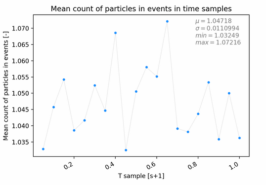
TimeSampling	FLOAT	Time in seconds for individual evaluations of the data sample -> the whole data sample and its time of collection is divided into sampling intervals with duration of the TimeSampling.	TimeSampling=1e-6 TimeSampling=0.00001 TimeSampling=233.2	1
DoMask	BOOL	Control to turn off masking if mask file is given.	DoMask=true DoMask=false	false

Detector Settings

It is possible to set the detector configuration with following list of parameters in the main parameters file:

• SensMat - sensor material (Si, CdTe, GaAs etc). Example: SensMat = "Si" to specify that the sensor material is silicon. Possible values:
  • Si - for silicon sensor. Used density:
  • CdTe - for cadmium teluride sensor. Used density:
  • GaAs - for galium arsenide. Used density:
• SensThick - Sensor thickness in micrometers. Example: SensThick = 500 to specify the thickness of the detector as 500 micrometers. This is continues variable.
• SensBias - sensor bias in volts. Example: SensBias = 100 to specify that applied was 100 V. This is a continues variable.
• ChipType - type of the chip (TPX or TPX3). Example: ChipType = "TPX3" to specify that TPX3 was used chip. Possible values:
  • TPX - for timepix chip
  • TPX3 - for timepix 3 chip
  • TPX2 - for timepix 2 chip
• SensDens - set density of used material in g/cm-3. DPE has default values for material specified in SensMat.

These values are used, for example, in the calculation of dose rate because there is a dependence on the sensor material and thickness. It also determines which PID algorithm should be used.

Input

Single File Processing

To process specific file with DPE, its name FILE_IN_NAME and path /PATH/TO /FILE/ must be specified via following parameters in parameters file:

    FileInName = "FILE_IN_NAME"
    FIleInPath = "/PATH/TO /FILE/"

This will cause that DPE will try to find this file and process it. Error is produced if the file can not be found and the processing is aborted.

Supported File Formats

The current version of the DPE engine is capable to process following files:

• Data driven files - t3pa, t3p, t3r
• Cluster log files- calibrated/uncalibrated
• Elist - only so-called full elist which includes also the header with cluster variables name.
• Frame formats

If a clog from itot+count measurement is used then it is needed to specify this in the main config file with following option:

    MeasMode = "itot+count"

Supported suffixes are following:

    ".t3pa", ".t3p", ".t3r", ".txt", ".pmf", ".plog", ".bmf", ".clog", ".elist", ".advelist", ".extelist"

Currently, the only toa formats are unsupported with undefined results deom DPE (time is handled as energy information).
Examples of most of the suported files can be found in the Examples/Test directory (list of examples is in the section First Example of Run)

Multi File/Batch Processing

It is possible to process several files in one run of DPE. There are several ways how to specify which files should be processed: * Process whole directory specifying path to the directory. * Process given files specifying their names in FileInName as an array. * Process only those files in directory which includes given strings in their names. Examples of such a processings can be found below.

Lets assume that our directory at path: /PATH/TO/DIR/ includes the following files: * File_001.t3pa * File_002.t3pa * File_003.t3pa * File.t3pa * File_2.clog

In the first case, when a whole directory should be processed, only the path to the directory is specified in the parameters file:

    FileInPath = "`/PATH/TO/DIR/"

DPE checks the existence of the directory and finds all files. It processes only those which have the same suffix/ending, and DPE found them first.
For this specific directory, let’s assume that File_001.t3pa was the first found by DPE, then all files ending with .t3pa are processed.
The file File_2.clog is not processed, because of the different suffix.
In the second case, when names of files are specified, it is needed to specify the names into parameter FileInName:

    FileInName = "File_001.t3pa", "File_003.t3pa", "File.t3pa"

DPE will process files: File_001.t3pa, File_003.t3pa and File.t3pa. Files with different suffixes should not be mixed! (e.g. clog and t3pa, DPE handles these files differently, which might cause unexpected behavior of the engine.)
In the last case, when user wants to specify only parts of the names, it is possible to specify beginning and ending of the name:

    FileInName = "File_"
    FileInNameEnd = "t3pa"

This will cause that only the following files are processed: File_001.t3pa, File_002.t3pa and File_003.t3pa. If only the first part of the name should be specified, there is need for one additional parameter DoMultiFile:

    FileInName = "File_0"
    DoMultiFile = true

DPE will again process the same list of files (additional 0 is needed due to the File_2.clog). In the opposite case when only ending of the name is specified, there is no need to add these parameters:

    FileInNameEnd = ".t3pa"

Files File.t3pa, File_001.t3pa, File_002.t3pa and File_003.t3pa will be processed.

The switch DoMultiFile can also be used to suppress multi file processing, setting it to false.

Output

Log and Print

During a run of the program, there is an output into the terminal. This include some basic information about the DPE settings and its run.
It can be turned off with DoPrint = false (default is true). Copy of this output is also given into log file, usually (default) called LogFile.txt. It can be turned off with DoLog = false (default is true). The preprocessing run of clusterer also created its own log file called log.txt where minimal log of clusterer run is stored.

Directory Tree

Results of DPE are exported into several directories separated in most cases based on the type of the analysis. There are some general directories for overall results. The creation of directories depends on used analysis and some of them might not be created if given processing is disabled or unsupported for given settings.

• File - main data files: elist, cluster log and sampling list. It is always created.
• Graph - graphical representation of the sampling list. Only if DoExportGraphics = true.
• Hist - histograms of cluster variables.
• SpatialMap - spatial maps of cluster variables also with respect to the PID classes.
• SigVec - significant vector which uniquely specifies the given radiation field.
• EventVisual - individual cluster plots, integrated sensor plots and plots of clusters for individual PID classes.
• Direction - results of directional analysis: estimation of radiation direction.
• CoincEvent - results of coincidence analysis: evaluates time correlation between clusters.
• Compton - results of coincidence analysis: evaluates time correlation between clusters.
• RadFieldRecog - results of coincidence analysis: evaluates time correlation between clusters.

These directories can have inner structure based on the specific exports of given analysis (export of graphs in directional analysis is done into directory Direction/Graph). More details can be found in the sections dedicated to these specifics analysis: directional, Compton, coincidence and radiation field recognition.
The whole export/output can be turned off if DoExportGraphics = false and DoExportText = false.

Text basic output

• Elist - file with cluster variables/parameters (this file is in default suppressed with DoRemoveElist = true and replaced with extended elist below).
• Extended Elist - elist extended with additional columns of PID class (-1 to N-1 of classes where -1 is for others, PIDClass) and filter pass (1 = passed, 0 = not passed, FilterPass) if the filter is used.
• Cluster log/clog - detailed list of clusters containing pixelated information. Each line which is starting with [ includes pixels of a cluster ([X,Y,E,T] = [X position,Y position,energy,time if tpx3 is sued] of a pixel). This file includes all clusters and the mask or filters are not accounted for.
• Sampling list - it includes basic information about the radiation field with respect to the observables and their time dependencies.
• Histograms - histograms of given variables - total and also for each PID class.
• Spatial maps - matrices of the sensor filled with integrated cluster variables (energy, size, LET, E/S).
• Significant vector - unique vectors characterizing processed radiation field computed based on histograms.
• Event and sensor visualizations - data files with matrices of exported clusters and sensor.

Each individual analysis also produces some parts of these results and more detailed descriptions are offered in dedicated sections below.

Graphical output

The current version uses a python scripts to convert the text output into graphics:

• Histograms
• Spatial maps
• Individual cluster plots (with values of the cluster variables) and integrated sensor plots
• Graphs of time evolution of physical products
• Directional maps
• Compton directional reconstruction
• …

For this purposes, the matplolib library is used. It can be slow for some configuration (for example high number of bins). To speed up the export of graphics, it is possible to set shown number of bins with following option:

    Hist1DGraphicsRebin = 100

which will cause that each histogram will be rebinned to show maximally 100 bins but the exported text files are still with the original number of bins. This option is only functional for 1D histograms.

Another possibility to speed up the plotting is the option DoGraphicsMultiThread which exploits several CPU threads for graphics creation. This option is by default on/true. The program then uses all threads on the given PC. To disable this feature use:

    DoGraphicsMultiThread = false

The multi processing can use up to several GB of ram memory which can be tuned with parameter GraphicsMultiThreadFileSize. Its default value is 3e6 and lower this number if the ram usage should be decreased (minimal ram usage is defined with needed ram for the biggest plot/histogram which can be of order of GBs).

To produce given plots, a directory .temp is created in the working directory. All python scripts are saved there before processing.
If the program is terminated just before or in the middle of graphics creation (python run) then a next run will firstly evaluate unfinished plotting and then proceeds with new plots therefore the whole plotting is delayed. In the case of sudden program abortion, it is recommended to check for existence of the .temp directory and delete it before the next run of DPE.

Clusterer and Preprocessing

The main purpose of this stage is to provide conversion of pixelated data into groups of correlated pixels, clusters. The level of correlation depends on the detector used for data collection. In the case of TPX detector, only spatial correlation is given and it is afterwards used for clusterization process. On contrary for the TPX3, time information is provided along the spatial one which gives opportunity to proceed with more precise clusterization process and eventually avoid additional unwanted effects as pile-up. At this stage main energy per pixel calibration is applied to convert digital ToT information to energy in keV. This process is accompanied with additional calibrations and corrections which aim to maximally supress detector unwanted or anomalous behaviour. The clusterization stage is followed with cluster analysis which evaluates clusters morphological and spectral features.

To summerize the pre-processeing stage:

• Clustering - grouping pixels based on coordinate and also on time information if given
• Calibration and corrections - energy calibration, cluster size correction, XRF peak suppression, TPX high energy correction etc.
• Cluster parameters - calculation of overall cluster parameters (total energy, roundness etc.)

Clustering

The clusterisation converts a frame or a continual stream of received pixels to sets of pixels which belonging to individual particles, clusters. A distinction is needed between two read out modes. In the case of the Timepix, the detector is only capable to measure in the frame mode and obtained data format is in a form of frames. The information is encoded into a sensor matrix of only hit pixels where each of them contain energy deposited during the acquisition time (if a measurement in ToT is performed¹). The same mode can be also used with the Timepix3 detector. The advantage with respect to the Timepix is the possibility to measure in the data driven mode. The final data output in this mode resembles the continual stream of pixels where time of arrival is stored together with deposited energy². This significantly improves the ability for the restoration of the individual particle information.

The algorithm used in the case of the frame mode relies only on the coordinate information. Pixels in a frame which are coordinate neighbours (lies within 8-pixel surroundings) are grouped together and called clusters:

It is also possible to measure in ToA mode, time of arrival or in a counting event mode.

In the case of combined ToT and ToA measurement which is another advantage of the Timepix3 with respect to the Timepix detector.

eq with clustering condition

During this clusterization process, an additional information about the readout can be used. It is known that the chip matrix of pixels is read out column by column which means that the stream of pixels can be efficiently parsed based on the column order. There are several disadvantages and crucial points concerning frame read-out:

1. Pile-up: All particles within one frame whose pixels are connecting cannot be separated within the clusterization process and they create the pile-up effect.
2. Loss of uncollected charge after the end of frame: It is possible that not all charge has been collected till the end of a frame (mostly some pixels with large deposited energy).
3. Dead time for matrix read out: This approximately several of millisecond (more than 10 ms).

These issues and disadvantages motivated development of the data-driven read-out mode. The coordinate information is accompanied by time of arrival which allows to reconstruct events also based on the time information. In this case, the stream of pixels is no longer separated into frames but it is continuously read by the read-out hardware and software.

In the first step, the stream has to time ordered because from the nature of the read-out, it is possible that the pixel stream violates time order. In the next stage, a block of pixels is taken from the full stream/list of pixels based on a time condition:

eq

The parameter should reflect expected time windows in the pixel stream and therefore is disproportional to particle fluence. The value is of order of . In those cases when the condition cannot be fulfilled, a fixed block of of pixels is taken. This number is approximately 100 000 pixels which should statistically minimized the error originating from possible separation of pixels belonging to one particle.

The clusterization process itself separates pixels into clusters based on two main conditions:

eq

These conditions can be translated as a need for pixels to be coordinate neighbours and to have maximal difference in time equal or less than time . The value of this time parameter is of order of tens of nanoseconds and it is dependent on the charge sharing effect and its magnitude.

Calibration and corrections

Energy calibration

Energy calibration of Time-Over-Threshold. Reprinted from Jakubek 2011.

After receiving the information from the detector, the possible energy and time of the detector are in corresponding ToT and ToA counts. These variables have to be calibrated and converted to obtain results in energy and time. Time conversion is done with following formula:

eq of toa conversion

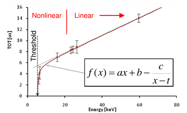
The first part of the calibration is the same for the Timepix and Timepix3 ASICs. This work was published by Jakubek and it is based on a combination of a linear and rational calibration function:

eq of calibrationwhere a,b,c and t are parameters obtained from the calibration procedure.

High Energy TPX Calibration

Histogram of measured energy before (light) and after (dark) application of the high energy calibration. Different biases were applied during the measurement to observe increase in the mean per pixel energy which has to be mainly corrected for (higher bias -> higher per pixel energy).

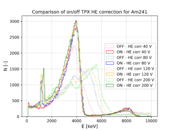
The calibration function has maximum of its validity up to approximately 700 keV for TPX. An additional per pixel calibration process has to be utilized for measurements in which higher per pixels energies are obtained. The additional calibration was intruced as a global model based on the results from the article of Sommer et al . Having the coefficients of the standard calibration and correlation matrix between these standards and the extended ones, it is possible to introduce an estimation of their values.

To use this additional calibration:

DoTpxHighEnergyCorr = true

The resulted histogram of the measured energy can be found in the fugere on the left. Two cases are shown in this image, before (light) and after (dark) an application of the high energy correction. Change in the sensor bias was also introduce during the measurement to demonstrate a different/increasing value of mean per pixel energy. Higher bias in the sensor decreases the effect of charge sharing and increases the per pixel energy and mainly the maximal per pixel energy of cluster. Therefore, it can be seen that in the most disturbed case of 200V the applied correction restores the original information to be in accordance with low bias measurement and their corrected versions.

In the case of TPX3, the energy range is limited with size of the ToT counter which has nominal value 1022. This means that the pixels cannot count more than 1022 counts in contrast to the TPX with counter range of 11810. From the practical point of view, the maximal value which can be measured in one pixel is between 450-500 keV (based on the settings of DACs). The standard energy calibration covers this region and a distortion appears for energy above 2 MeV as the volcano effect.

Cluster Energy Size Based Correction

...

Halo Effect

...

Correction for XRF peak suppression

...

Pile-up Recognition

...

Volcano Effect

Heavy ion cluster in energy plot with a direction almost perpendicular to the sensor plane. Two additional sensor effects can be observed: the volcano and the halo effect.

... Source

Overshoot

...

Time-walk Correction

... Source

Cluster Variables and Elist

• The file includes clusters/events represented as a set of cluster variables.
• The significant feature of the Elist is a presence of coincidence group expressed as coincidence number and it is adjustable based on the coincidence time interval.

LengthCorrStd	Unit	Column	Description
DetectorID	-	1	It serves to as a unique ID in the cases when multi detector setup is processed.
EventID	-	2	ID of events. In the case that several clusters are in the coincidence, then they have the same EventID. It starts from 0 and clusters which are not in coincidences are also accounted in this ID.
X	px	3	X coordinate of cluster based on the weighted mean value of X coordinate of pixels, weighted with the energy of pixels. Value ha range from 0.5 to 255.5 (minimal and maximal value of X of pixels).
Y	px	4	Y coordinate of cluster based on the weighted mean value of Y coordinate of pixels, weighted with the energy of pixels. Value ha range from 0.5 to 255.5 (minimal and maximal value of Y of pixels).
E	keV	5	Energy of cluster, also called volume. It is sum of energies of all cluster pixels.
T	ns	6	Time. It is the minimal time of cluster pixels.
Flags	-	7	Free column for user needs. In the case of frame data, it includes frame number.
Size	px	8	Count of cluster pixels.
Height	keV	9	Maximal value of energy of cluster pixels.
BorderPixCount	px	10	Count of border pixels in cluster.
Roundness	-	11	Morphological feature expressing similarity of cluster to round shape.
AngleAzim	deg	12	Estimation of
Linearity	-	13	Morphological feature expressing similarity of cluster to linear shape.
LengthProj	px	14	Length of cluster based on maximal distance between pixels after projection to the cluster axis.
WidthProj	px	15	Length of cluster based on maximal distance between pixels after projection to the axis perpendicular to the cluster axis.
IsSensEdge	-	16	Information whether cluster is at sensor edge. 0 for flase, 1 for true (is at sensor edge).
StdAlong	px	17	Weighted standard deviation of pixels with respect to cluster axis weighted with pixels energy.
StdPerp	px	18	Weighted standard deviation of pixels with respect to axis perpendicular to the cluster axis and weighted with pixels energy.
Thin	-	19	Morphological feature expressing thinness of cluster.
Thick	-	20	Morphological feature expressing thickness of cluster.
CurlyThin	-	21	Morphological feature expressing combination of cluster thinness and inverse of linearity.
EpixMean	keV	22	Mean value of pixels energy in cluster.
EpixStd	keV	23	Standard deviation of pixels energy in cluster.
LengthCorrStd	px	24	Cluster length in sensor plane corrected for charge sharing based on weighted standard deviation.
Length3DCorrStd	um	25	Cluster length in sensor volume corrected for charge sharing based on weighted standard deviation.
LengthCorrWidth	px	24	Cluster length in sensor plane corrected for charge sharing based on cluster width.
Length3DCorrWidth	um	25	Cluster length in sensor volume corrected for charge sharing based on cluster width.
LengthCorrNabha	px	24	Cluster length in sensor plane corrected for charge sharing based on Nabha model.
Length3DCorrNabha	um	25	Cluster length in sensor volume corrected for charge sharing based on Nabha model.
AngleElev	deg	26	Elevation angle of cluster.
LET	keV/um	27	Linear energy transfer based on the corrected length and energy (E).
Diameter	px	28	...
PIDClass	-	29	If PID is used, this number expressed class into which the cluster was classified. It goes from 0 to count_class - 1.
FilterPass	-	30	If filter is used, then it includes information whether cluster passed given filters or did not. 1 for passed, 0 for did NOT pass.

Example of created elist:

Cluster log

Clusters can be exported as individuals pixels. This format is called cluster log or clog and it is highly dependent on the input data (detector, measured mode, etc.). In the case of TPX detector the format is following:

Frame 1 (UNIX_TIME, ACQ_TIME s)
[X_1, Y_1, iToT_1/E_1/] [X_2, Y_2, iToT_2/E_2/]...
....

Frame 2 (UNIX_TIME, ACQ_TIME s)
[X_1, Y_1, iToT_1/E_1] [X_2, Y_2, iToT_2/E_2]...
....

where ACQ_TIME is acquisition time of frames and UNIX_TIME is current UNIX time stamp in seconds (both). Every line starting with [ is one cluster and in each square brackets is one pixel and its information [x coordinate,y coordinate, iToT/Count/Energy]. The ToA and Count modes are not correctly implemented and they are treated as the ToT mode (especially of importance for the cluster parameters in the elist).

The format is different for the TPX3 detector:

Frame 1 (FIRST_TIME_COINC_GROUP, COINC_TIME_WINDOW ns)
[X_1 ,Y_1, ToT_1/E_1, T_Diff_1] [X_2, Y_2, ToT_2/E_2, T_Diff_2]...
[X_1 ,Y_1, ToT_1/E_1, T_Diff_1] [X_2, Y_2, ToT_2/E_2, T_Diff_2]...
.... 

Frame 2 (FIRST_TIME_COINC_GROUP, COINC_TIME_WINDOW ns)
[X_1 ,Y_1, ToT_1/E_1, T_Diff_1] [X_2, Y_2, ToT_2/E_2, T_Diff_2]...
[X_1 ,Y_1, ToT_1/E_1, T_Diff_1] [X_2, Y_2, ToT_2/E_2, T_Diff_2]...
....

where each frame in this case coincidence group = clusters whose min times are within the COINC_TIME_WINDOW starting with the first one at FIRST_TIME_COINC_GROUP. The pixels time is written as difference with the FIRST_TIME_COINC_GROUP: T_Diff = T_Pix - FIRST_TIME_COINC_GROUP where T_Pix is original time of pixels in ns. An exception from this rule is measurement in the frame mode iToT+Count when data are already saved in cluster log within the Pixet. To properly evaluate this data with the clusterer, it is needed to add additional option into the command line:

--measmode "itot+count"

This data does not include additional ToA information therefore the format has the same meaning as in the first case with TPX:

Frame 1 (UNIX_TIME, ACQ_TIME s)
[X_1 ,Y_1, iToT_1/E_1, Count_1] [X_2, Y_2, iToT_2/E_2, Count_2]...
[X_1 ,Y_1, iToT_1/E_1, Count_1] [X_2, Y_2, iToT_2/E_2, Count_2]...
.... 

Frame 2 (UNIX_TIME, ACQ_TIME s)
[X_1 ,Y_1, iToT_1/E_1, Count_1] [X_2, Y_2, iToT_2/E_2, Count_2]...
[X_1 ,Y_1, iToT_1/E_1, Count_1] [X_2, Y_2, iToT_2/E_2, Count_2]...
....

Summary of supported input data formats: * TPX3, data driven mode, tot+toa * TPX3, frame mode, itot+count * TPX, frame mode, tot Every other format will be processed but the results might be uncorrected evaluated, for example in the cluster parameters.

Reprocessing of cluster logs can create cluster logs which could have incorrect coincidence group (in the case of TPX3 with ToA). If the coincidence window el-coinctoadiff is increased with respect to the original one then the resulted group will not integrate several groups together which would fulfill this new time condition.

Masking

There is a possibility to mask a part of the sensor or individual pixels in the case of t3pa and clog files.
These pixels are omitted in the pre-processing.
This can be used to avoid a signal from noisy pixels or to focus on some more interesting part of the sensor.
The configuration is done through a configuration file. An example can be found in the program directory.
If the masking is used the during the pre-processing an additional t3pa/clog file is created with masked pixels according to the user configuration in the export directory (starts with MASK_+ FileInName).

Inclusion of Mask.ini into Parametrs File

The configuration file of the mask can be included with following options in the ParametersFile:

    MaskName = "Mask.txt"       // Name of the INI configuration file of the mask.  
    MaskPath = "PATP/TO/MASK/"  // Path of the INI configuration file of the mask.

Syntax of Configuration File

• The pixel which should be masked is written in format [X,Y]. These are X and Y coordinates of the pixel where both of them are integers from 0 to 255. The sensor orientation is usual and X coordinate is for rows and Y is for lines. They can be written in lines or rows in the mask file but always the [X,Y] in one line (can not be separated over several lines)
• If a larger part is of interest, following notation is used: [X_min - X_max, Y_min - Y_max] where X_min is the minimum coordinates of a pixel, X_max is the maximum coordinate of a pixel etc. For example, [0-255,0-120] masks almost half of the sensor - on the X axis from 0 to 255 and on the Y axis from 0 to 120. A simpler demonstration can be masking of one line of pixels (11th) : [0-255, 10].

Example of all possibilities for masking:

    [0,1] [2,5]
    [2,3]

    [2-43,5]
    [76,8-90]
    [0-50,50-60]

Masking with Pixet Mask

It is also possible to exploit the masking created in Pixet, which takes the form of a text file where the lines and rows correspond to those of the detector. The orientation in this case is the same for x axis, but it is reversed for y axis where bottom of the detector is first line and top part of the detector is last line. The delimiter in this case is simple white space . The masked pixels are marked as 0 and unmasked are 1. See following example (... used as abbreviations):

    1 1 1 1 0 1 ... 1
    1 1 1 1 1 1 ... 1
    ...
    0 1 1 1 1 1 ... 1

Statistical Information

Statistical information can be found in the general sampling list and it is also printed into log.
Example for the sampling list in json format (explanations are given in the comments after //):

    "CountPixHit_Sum_MaskOk_cnt":242461,    // Count of pixels which passed the mask and used for processing.  
    "CountPixHit_Sum_MaskOk_perc":99.23,    // The same as above but as part/percentage to total amount of pixels.
    "CountPixHit_Sum_MaskOmit_cnt":1872,    // Count of pixels which did NOT pass the mask and they are used for processing.  
    "CountPixHit_Sum_MaskOmit_perc":0.766,  // The same as above but as part/percentage to total amount of pixels.
    "CountPixHit_Sum_All_cnt":41935,        // Total count of loaded pixels for raw data.

Example for log file:

    Mask conf file - name:      Mask.txt
    Mask conf file - path:      ./Test/data/test_029/

    ...

    --------------------------------------------------
    SENSOR MASK
        ...has been loaded.

    Count of masked pixels:     901 (1.37%)
    --------------------------------------------------

    ...

    Processing RawData T3PA:    
    Creating masked raw file:   MASK_tot_toa.t3pa

    ...

    --------------------------------------------------
    MASK
    --------------------------------------------------

    CountPixHit_Sum_MaskOk [-]:   242461
    CountPixHit_Sum_MaskOk [%]:   99.23
    CountPixHit_Sum_MaskOmit [-]: 1872
    CountPixHit_Sum_MaskOmit [%]: 0.766
    CountPixHit_Sum_All [-]:      41935

First part shows from which destination is the mask taken and what is the name of the file.
The second part informs about successful loading of the file and how many pixels are masked.
The third part appears in the preprocessing sections and informs about actual masking of the raw data.
The last part is in the sections with results and includes the same information as it is in the sampling file.

Filtering

During the processing, filters can be used to obtain only information about particles of interest.
The filters are applied on cluster variables/parameters level (e.g. energy, height etc.). It is specified trough a configuration file in the INI format.
The cluster variables which should be used for filtering are specified with their unique name which is included
in the header of the created elist (if elist is input then it has to be already part of the file).
All results produced by DPE are only for filtered particles/for those which passed filter (histograms, graphs, spatial maps etc.).
An example can be found in the program directory.

Inclusion of Filter.ini into Parameters File

The configuration file of the filter can be included with following options in the ParametersFile:

    FilterName = "Filter.ini"           // Name of the INI configuration file of the filter.  
    FilterPath = "/PATH/TO/FILTER/"     // Path of the INI configuration file of the filter.

Syntax of Configuration File

The configuration file in INI format is a set of sections where each section is dedicated to one cluster parameter for which filtering should be done.
Individual parts of these sections are specific values of the filters for the given cluster parameter. Example with filter conditions for energy of clusters alias row E in elist:

• One section of the configuration file is named based on the key E in the elist: [E].
• Condition is then written as Range=100,200. The name Range has to be first part of the condition name. This settings will produce a filter on cluster energy which should be only from 100 to 200 keV (edges are included).
• More ranges can be specified for one parameter. Individual conditions/ranges have to always include string Range in names, but they have to differ, therefore suffixes/endings have to be introduced: Range_1, Range_2 etc. (, see example below).

Filter with single condition in energy E from 100 to 200 keV:

    [E]
    Range = 100, 200   

Filter with multiple conditions on energy E:

    [E]
    Range_1=100,200  
    Range_2=500,1000  
    Range_asdasd=300,2000  

Names of Cluster Parameters/Variables

The valid names are enclosed in the quotations (e.g. DetectorID to filter based on detector ID):

    #define CL_PAR_DET_ID          "DetectorID"
    #define CL_PAR_EVENT_ID        "EventID"
    #define CL_PAR_FLAG            "Flags"
    #define CL_PAR_X_E             "X"
    #define CL_PAR_Y_E             "Y"
    #define CL_PAR_Z               "Z"
    #define CL_PAR_E               "E"
    #define CL_PAR_H               "Height"
    #define CL_PAR_S               "Size"
    #define CL_PAR_T_MIN           "T"
    #define CL_PAR_N_BORD_PIX      "BorderPixCount"
    #define CL_PAR_ROUND           "Roundness"
    #define CL_PAR_DIAMETER        "Diameter"
    #define CL_PAR_LIN             "Linearity"
    #define CL_PAR_THIN            "Thin"
    #define CL_PAR_THICK           "Thick"
    #define CL_PAR_CURLY_THIN      "CurlyThin"
    #define CL_PAR_ANGLE_AZIM      "AngleAzim"
    #define CL_PAR_ANGLE_ELEV      "AngleElev"
    #define CL_PAR_EPIX_MEAN       "EpixMean"
    #define CL_PAR_EPIX_STD        "EpixStd"
    #define CL_PAR_LET             "LET"
    #define CL_PAR_W2D_PROJ        "WidthProj"
    #define CL_PAR_L2D_PROJ        "LengthProj"
    #define CL_PAR_L2D_CORR_STD    "LengthCorrStd"
    #define CL_PAR_L3D_CORR_STD    "Length3DCorrStd"
    #define CL_PAR_L2D_CORR_WIDTH  "LengthCorrWidth"
    #define CL_PAR_L3D_CORR_WIDTH  "Length3DCorrWidth"
    #define CL_PAR_L2D_CORR_NABHA  "LengthCorrNabha"
    #define CL_PAR_L3D_CORR_NABHA  "Length3DCorrNabha"
    #define CL_PAR_SENS_EDGE       "IsSensEdge"
    #define CL_PAR_STD_ALONG       "StdAlong"
    #define CL_PAR_STD_PERP        "StdPerp"
    #define CL_PAR_PID_CLASS       "PIDClass"

The PIDClass is created during processing as result of the particle identification.

Output into Extended Elist

The output of the filtering can be found in the extended elist (in directory File). New column is created with name FilterPass.
The values of this new clomun/parameter are 1 for passing the filter and 0 for NOT passing the filter.
All particles are stored in the extended elist, but it is possible to suppress the export of those particles which did not pass the filter conditions:

DoExportElistExtFilter = false

with this switch in the parameters file, only those particles which passed the filter are exported into extended elist (column FilterPass is still present).

Statistical and Log Information

Statistical information can be found in the general sampling list and it is also printed into log.
Example for the sampling list in json format (explanations are given in the comments after //):

    "CountParticle_Sum_FilterOk_cnt":4386,      // Count of particles which passed the filter.
    "CountParticle_Sum_FilterOk_perc":58.93,    // Percentage of the above to the total count of particles.
    "CountParticle_Sum_FilterOmit_cnt":3057,    // Count of particles which did NOT pass the filter.
    "CountParticle_Sum_FilterOmit_perc":41.07,  // Percentage of the above to the total count of particles.
    "CountParticle_Sum_All_cnt":7443,           // Count of all particles which were evaluated.

    Filter conf file - name:    Filter.ini
    Filter conf file - path:    ./Test/data/test_007/

    ...

    --------------------------------------------------
    FILTER

    Conditions are logically connected as AND for different variables (within always as AND)

        INDEX|NAME        CONDITIONS [min|max]

        10|Roundness
         |-----------[0|2]
         '-----------[0.4|0.45]
        9|BorderPixCount
         |-----------[1|10]
         '-----------[20|1e+200]
        4|E
         '-----------[100|1e+300]
    --------------------------------------------------


    ...


    --------------------------------------------------
    FILTER
    --------------------------------------------------

    CountParticle_Sum_FilterOk [-]:         4386
    CountParticle_Sum_FilterOk [%]:         58.93
    CountParticle_Sum_FilterOmit [-]:       3057
    CountParticle_Sum_FilterOmit [%]:       41.07
    CountParticle_Sum_All [-]:              7443

The first part informing about name and path to the config file of filter can be seen in the first stage of DPE processing.
The second part is in the same processing/nationalization stage of DPE and it shows which filter were recognized and what ranges are about to be used.
The last part informs about statistical information and it includes the same information which are also given in the json sampling list.

Histograms

One of the DPE outputs are histograms of cluster variables/parameters.
The DPE in default exports 1D histograms of all cluster variables in extended elist and also several their combinations as 2D histograms.
It is possible to export user defined 1D and 2D histograms which can be configured with a configuration file in the INI format (an example can be found in the program directory).
The DPE allows to also create histograms of algebraic combinations of the cluster variables (multiplication, division, subtraction, addition).
It is important that the general label (key name of a section in a INI file) of the histogram used in the INI file is unique to each histogram.
If there are more histograms with one common name then the program only updates information about the first one in the INI file.
The label itself in not used in the program itself and title and name of the histogram are set separately.
The histograms are used in other analysis, therefore their changes/using user configuration might disturb e.g. creation significant vectors. This might produce following error for significant vectors:

[ERROR] -1041 : Error occurred during significant vector module initialization. Module will not be used in processing.

It just informs that the settings of histograms is not compatible with settings of significant vectors.

Inclusion of Hist.ini into Parameters File

To use user configuration file for histograms, it is needed to add two parameters into paramters file, name (e.g. Hist.ini) and path (e.g. PATH/TO/HIST/CONFIG/) to the configuration file:

HistName - "Hist.ini"               // Name of the configuration file for histograms.
HistPath = "PATH/TO/HIST/CONFIG/"   // Path of the configuration file for histograms.

If at least the name is set and the file is found on the given location then the DPE uses this settings of histograms otherwise default configuration is used.

Histogram 1D

The 1D histograms can be created as fixed bin width histograms or with variable binning (different width of bins).
Lets assume that histograms of size should be created Hist1D_Size.
The fixed bin width has following settings/needed parameters (example from configuration file with explanations = everything after #):

    [Hist1D_Size]

    VarName="Size"  # Name of column with given variable (see the first line in Elist.txt - it has to be the same)
    Title="S"       # Title of histogram (can be arbitrary - X if not given)
    NBin=9          # Number of bins 
    Xmin=100        # Minimum value (if X = Xmin -> it is NOT included to the first bin - it has to be > Xmin)
    Xmax=1000       # Maximum value (if X = Xmax -> it is included to last bin NBin)

The same as above but with different choice of variable, it is based on the column position in the elist instead of the cluster variable name:

    [Hist1D_Size]

    ColIndex=7      # Position of the column - starts from 0 (it is Size in the example)
    Title="S"       # -||-
    NBin=9          # -||-
    Xmin=100        # -||-
    Xmax=1000       # -||-

These cases create histogram from cluster size with 9 bins from 100 to 1000 where one bin has width 100. Variable size bin width and its needed parameters (same histogram as the one above):

    [Hist1D_Size]

    VarName="Size"  # -||-
    Title="S"       # -||-
    BinLowEdge=100,200,300,400,500,600,700,800,900,1000     # Low edges of bins with Xmax (Xmin,...,Xmax -> size NBin+1)        

Histogram 2D

The 2D histograms are constructed in similar manner as 1D histograms. The fixed bin width histograms and their needed parameters:

    [Hist2D_SE]

    VarName="E","Size"  # Name of columns with given variable - 1st is X, 2nd is Y (see the first line in Elist.txt - it has to be the same or see special variables)
    Title="E,S"         # Title of histogram (can be arbitrary - X if not given)
    NBinX=9             # Number of X bins where X is in this case energy,E
    Xmin=100            # Minimum value of X (if X = Xmin -> it is NOT included to first bin - it has to be > Xmin)
    Xmax=1000           # Maximum value of X (if X = Xmax -> it is included to last bin NBin)
    NBinY=1000          # Number of Y bins 
    Ymin=0              # Minimum value of X (if X = Xmin -> it is NOT included to first bin - it has to be > Xmin)
    Ymax=1000           # Maximum value of X (if X = Xmax -> it is included to last bin NBin)

An example for cluster variables based on column positions in the elist:

    [Hist2D_SE]

    ColIndex=4,7        # Position of the columns which should be processed - 1st is X, 2nd is Y 
    #...(the same as above) 

These cases create 2D histogram of cluster energy and size where energy is from 100 to 1000 with bin width of 100 and size is from 0 to 1000 with bin width of 1. Variable size bin width and its needed parameters:

    [Hist2D_SE]
   
    VarName="E","Size"  # -||-
    Title="E,S"         # -||-
    BinLowEdgeX=100,200,300,400,500,600,700,800,900,1000    # Low edges of X bins with Xmax (Xmin,...,Xmax -> size NBinX+1)     
    BinLowEdgeY=100,200,300,400,500,600,700,800,900,1000    # Low edges of Y bins with Ymax (Ymin,...,Ymax -> size NBinY+1)     

It is also possible do just variable binning in one variable the second one can be with fixed bin size:

    [Hist2D_SE]
   
    VarName="E","Size"      
    Title="E,S"             
    NBinX=9             
    Xmin=100                
    Xmax=1000               
    BinLowEdgeY=100,200,300,400,500,600,700,800,900,1000         

Additional Algebraic Operations

Both 1D and 2D histograms allow additional operations of addition, subtraction, multiplication and division on extracted variables from EList.

Histogram 1D:

    ColIndex_Div=4,7    # Division as 5th/7th column (in this case E/S = Epix) - 1st argument is divided by 2nd argument
    ColIndex_Mult=4,7   # Multiplication as 5th*7th column - 1st argument is multiplied with 2nd argument 
    ColIndex_Add=4,7    # Additions 5th+7th column- 1st argument is added to 2nd argument
    ColIndex_Subtr=4,7  # Subtraction as 5th-7th column - 2nd argument is subtracted from 1st argument

An example based on cluster variable names:

    VarName_Div="E","Size"  # Same thing as above but with names of columns
    VarName_Mult="E","Size" # Same thing as above but with names of columns
    VarName_Add="E","Size"  # Same thing as above but with names of columns
    VarName_Subtr="E","Size"# Same thing as above but with names of columns     

Histogram 2D:

Very similar to 1D histograms but always the first given is X and the second given is Y.

    ColIndex=4              # X is set to 4th column - energy
    ColIndex_Div=4,7        # Y is set to division of 4th/7th

Operations used for both variables:

    ColIndex_Div=8,7,4,7    # X is set to division of 8th/7th and Y is set to division of 4th/7th

The same thing can be done with names of columns/variables VarName:

    VarName_Div="E","Size","Height","Size"  # X is E/Size and Y is Height/Size

Text export

There are two kinds of exported files: histogram data and histogram information/info file.
The histogram data file includes content of bins and bins low edges. The histogram info file comprehends features of the histogram: title, name, count of bins etc. (see more details below).
The data file has a suffix .hist and the info file .hist_info. The data file has following formatting for 1D histogram:

    Xmin              BinCont_1
    BinLowEdge_2      BinCont_2     
    ...               ....
    BinLowEdge_NBin   BinCont_NBin
    Xmax              Overflow

The Xmax is included to allow an user easier read of this file without direct need to also read the info file (all needed information is in the data file in the base case).
It is also possible to export only those bins which have non zero content with fixed binning. This can be done with following option in the Hist.ini file:

DoSparseExport=1    # Check whether only nonzero bins should be exported (1 for true and 0 for false).

It has to be used for each histogram separately and it is used as default settings. The exported data file has following format:

    Xmin              BinCont_1   
    BinLowEdge_2      BinCont_2   
    ...               ...
    BinLowEdge_i      BinCont_i != 0
    ...               ...
    Xmax              Overflow 

The Xmin,BinLowEdge_2,Xmax are always exported even if their bin content is 0 for further reading and reconstruction of histograms. This option is not functional for variable binning to avoid a lack of information in the data file for histogram complete reconstruction in post-processing. To reconstruct the histogram, it can be done just based on the data file even in the case of sparse export because the missing bins
and bin width can be calculated based on the first two bins in the data file (BinWidth = BinLowEdge_2 - Xmin).
Anyway, it is recommended to read the info file for example in the case of constant bin width combined with the sparse export to ensure that given
histogram is truly with constant binning and not variable binning (written in the parameter: BinEquiDist=1 = it is const binning and 0 for variable binning).

Similar approach is utilized for the 2D histograms:

    Xmin                Ymin                BinCont_1                   # First bin
    XBinLowEdge_2       Ymin                BinCont_2     
    ...                 ....                ....
    XBinLowEdge_NBinX   Ymin                BinCont_NBinX     
    Xmin                YBinLowEdge_2       BinCont_NBinX+1
    ...                 ....                ....
    XBinLowEdge_NBinX   YBinLowEdge_2       BinCont_NBinX+NBinY   
    XBinLowEdge_2       YBinLowEdge_3       BinCont_NBinX+NBinY+1           
    ...                 ....                ....
    XBinLowEdge_NBinX   YBinLowEdge_NBinY   BinCont_NBinX*NBinY         # Last bin               
    Xmax                Ymax                Overflow

The sparse export has following form.

    Xmin                Ymin                BinCont_1
    XBinLowEdge_2       Ymin                BinCont_2     
    ...                 ....                ....
    XBinLowEdge_i       Ymin                BinCont_i != 0   
    ...                 ....                ....
    Xmin                YBinLowEdge_2       BinCont_NBinX+1
    ...                 ....                ....
    XBinLowEdge_m       YBinLowEdge_n       BinCont_m+n*NBinX != 0           
    ...                 ....                ....
    Xmax                Ymax                Overflow

It is similar to 1D histogram with the exception that there is also the next Y low bin edge to also estimate the width of binning for Y axis.

The info file is formatted as an INI file and it includes the same information as the Hist.ini file for each histogram individually. There two additional features compared with the Hist.ini:

• Statistical information (mean, err of mean, std, err of std)
• Overflow and underflow information

Explanation of individual parameters are written as comment in example below:

    [HistPar]

    Title="Hist1D_Epix_1"                       # Title of the histograms used for unique recognition 
    Name="Mean energy per pixel of cluster"     # General name 
    AxisTitles="Epix [keV/px]","N [-]"          # Names of axis titles/lables.
    NBin=300                                    # Count of bins
    Xmin=0                                      # HIstogram minimum
    Xmax=300                                    # Histogram maximum
    BinEquidist=1                               # Check whether histogram has same width bins

    [HistCont]

    Underflow=0                                 # Count all events which are below Xmin 
    Overflow=1                                  # Count all events which are above Xmax

    [Statistics]

    Mean=29.6869                                # Estimation of weighted mean value of histogram (weighted with bin contents) 
    Mean_Err=0.20951                            # Error of the mean estimation
    Std=13.9273                                 # Estimation of weighted standard deviation of histogram (weighted with bin contents) 
    Std_Err=1.40088                             # Error of the std estimation

Equivalent information is also given for histogram 2D with appropriate extension of additional dimension.

Graphical export

Derived deposited energy histograms with equidistant binning. Data displayed in lin scale (top plot) and log scale (bottom plot).

There is possibility to create plot of Hist1D and Hist2D via python matplotlib, it has to be preinstalled.
The current version will automatically create these plots if DoExportGraphics=true but it can be turned off - see below.

    SOME_PREVIOUS_CODE                  # This is some code to call histogram 2D
    Name="Histogram2D title in plot"    # Name o histogram in plot
    AxisTitle="X","Y","N"               # Name of axis in the plot

The plots can be with logarithmic scales on all axis:

    SOME_PREVIOUS_CODE      # This is some code to call histogram 2D
    DoLogX=1                # 1 for true=do logarithmic X axis and 0 for false
    DoLogY=1                # 1 for true=do logarithmic Y axis and 0 for false

To turn off plotting:

2D histogram of cluster size and energy. The figure is accompanied with statistical information about mean values, standard deviations, sum/integral, maximum and minimum value.

    SOME_PREVIOUS_CODE  # This is some code to call histogram 2D
    DoPlot=0            # Default is 1 - do plot and 0 means not do plot

It is possible to adjust the number binning of the histogram only for the graphics. This can be done with Hist1DGraphicsRebin in the main configuration file:

    Hist1DGraphicsRebin = 100

This option with value 100 will change the shown number of bins in the graphics to 100 but the exported files includes original binning.
This is allowed for faster exports of histograms with more than 10000 bins which can time challenging for a PC.

Log Information

    Hist conf file - name:      Hist.ini
    Hist conf file - path:      ./Test/data/test_006/

    ...

    --------------------------------------------------
    HISTOGRAMS

    1D:
        Hist1D_E_Total from column 4
        Hist1D_S_Total from column 7
        Hist1D_LET_Total from column 26
        Hist1D_EpixMean_Total from column 21
        Hist1D_Epix_Total from column-division: 4/7
        Hist1D_H_Total from column 8
        Hist1D_LET_VarBinWidth_Total from column 26
    2D:
        Hist2D_ES_Total from column 4 7
        Hist2D_ES_VarBinWidth_Total from column 4 7

    --------------------------------------------------

    ...

    Hist are be shown with max N bins:  100 bins

    ...

    Exporting histograms to: ./Test/out/test_006/./Hist/

        Exporting histogram 1D: Hist1D_E_1
        Exporting histogram 1D: Hist1D_S_1
        Exporting histogram 1D: Hist1D_LET_1
        Exporting histogram 1D: Hist1D_EpixMean_1
        Exporting histogram 1D: Hist1D_Epix_1
        Exporting histogram 1D: Hist1D_H_1
        Exporting histogram 1D: Hist1D_LET_VarBinWidth_1
    ...

The first part informing about name and path to the config file of histograms can be seen in the first stage of DPE processing.
The second part is in the same processing/nationalization stage of DPE and it shows which histograms will be produced.
The last tow parts informs exporting of histograms (first one only if change of hist binning is used in graphical plots).

Significant Vectors

The significant vectors is a unique set/vector of numbers which describes given data sample/radiation field.
It can be used for radiation field recognition as it is done in the DPE.
There is a possibility to create own configuration file for the generation of the significant vector.
The significant vectors are exported into directory SigVec in path FileOutPath.
The analysis/generation of SigVec can be suppressed with the following option in Parameters file:

DoSigVec = false

The results are saved into directory SigVec into files SigVec.vec and SigVec.vec_info. First file includes the vector itself and second file includes information about the vector (used histograms, intervals etc.).

Theoretical Introduction

The significant vectors are sets of numbers which should describe uniquely a radiation field. They are created form 1D and 2D histograms based on the following rules (see the illustrations in the ):

1. 1D histograms: Each number of the significant vector is produced as a sum of bin contents within some specified ranges. Assuming that some elements of the vector should be done based on the energy distribution/histogram. Ranges of interests have to be specified where an integration is executed. This specification of the ranges is a task for an optimization method and differentiates based on the set of radiotin fields which should be recognized. One number is created for each range. These are normalized with a total integral over whole histogram to achieve comparability with different fields where more or less particles could be measured. A weighting can be also introduced as a last stage of the process to highlight some elements of the vector. This procedure can be done for several other cluster variables resulting in the vector of significant variables.
2. 2D histograms: Their conversion into significant variables obey similar rules as the 1D histograms. Except for the ranges, masks can be also specified which determines the area of interest. The integration is based on this mask where the mask has the same features as the histogram itself with values which can be used as weights. The mask values are used as a multiplicative factor in the integration therefore bins with 0 are ignored and bins with value higher than 1 are highlighted.

Inclusion of SigVec.ini into Parameters File

The the DPE will include a user configuration file only if it is written in the PararamtersFile.
Two parameters are used for this purpose (assume that name of config file is SigVec.ini in path /PATH/TO/SIGVEC/CONFIG/):

    SigVecName = "SigVec.ini"                  // Name of the configuration file for significant vectors.
    SigVecPath = "/PATH/TO/SIGVEC/CONFIG/"     // Path to the configuration file for significant vectors.

If at least the name is set and the file is found on the given location then the DPE uses this settings of SigVec otherwise default configuration is used.

Histogram 1D - Intervals of Interest

A histogram is examined and all bins (bin contents) with bin center between up and down edge/limit of given interval is summed, number R_1.
This number is used as one element of SigVec = {R_1, R_2, … , R_N} for N of intervals.
At least two numbers has to be given - down and up edge of the interval where interval condition for bins are following: DOWN_EDGE < BinCenter <= UP_EDGE.
An example of configuration file for 1D histogram:

    [Var_Epix]                          # Section name as unique key of the given SigVec element. It has to include the string "Var_".

    Title="Epix"                        # Title of the variable.
    HistName="Hist_Epix"                # Name of histogram which should be processed - same as name of histogram file without suffix/ending in directory Hist (data suffix)
    Intervals=0,200,100,500,500,5000    # Limits of intervals - 1st interval = from 0 to 200, 2nd interval = from 100 to 500 etc. (N in this case is 3)

The intervals can be overlapping. The section name has to include string Var in its name and they have to differ for different elements of the SigVec: Var_E, Var_S, ....

Histogram 2D - Regions of Interest

A histogram is multiplied with mask (from 0 val to inf - can serve as weights) with the same number of bins.
Then the histogram is summed and this number is as an input to the SigVec.
For each given mask one number is produced. An example of configuration file:

    [Var_E_S]                               # Section name as unique key of the given SigVec element. It has to include the string "Var_".

    Title="E_S"                             # Title of the variables
    HistName="Hist_E_S_2"                   # Name of histogram which should be processed - same as name if histogram file without suffix/ending in directory Hist (data suffix)
    Mask_1="\PATH\TO\MASK\MASK1_FILE_NAME"  # Path to masks which should be applied - same dimensions as histogram (see examples)
    Mask_2="\PATH\TO\MASK\MASK2_FILE_NAME"  # Path to masks which should be applied - same dimensions as histogram (see examples)

Lets assume that the Hist_E_S_2 is following histogram: NBinX = 5, Xmin = 0, Xmax = 10 & NBinY = 4, Xmin = 0, Xmax = 4 then the mask should have following form:

0 1 0 0 0
0 0 0 0 0
0 2 0 0 3
0 0 0 4 10

A single gap is used as number separator.This will use bins [X,Y,Weight] = [2,1,1], [2,3,2], [5,2,3], [4,4,4], [4,5,10] and the matrix is read from first line to the last one (1st line is Y = 1).

Normalization

Both 1D and 2D histograms can be normalized before they are used calculation of the SigVec:

    Normalize=1         # 1 to DO normalization - 0 to NOT do norm. - default is 0

Default Configuration

    [Var_S]

    Title="Var_S"
    Intervals=-1,5,5,20,20,1e+200
    Normalize=1

    [Var_BorderPixN]

    Title="Var_BorderPixN"
    Intervals=-1,2,2,5,5,15,15,1e+200
    Normalize=1

    [Var_Lin]

    Title="Var_Lin"
    Intervals=-1,0.5,0.5,0.95,0.95,1e+200
    Normalize=1

Minimum values -1 and maximum 1e+200 are safety precautions to be sure that all relevant bins are taken into account.

Log Information

    SigVec conf file - name:    SigVec.ini
    SigVec conf file - path:    ./Test/data/test_008/

    ...

    --------------------------------------------------
    SIGNIFICANT VECTOR

    Features:

        Title = Epix 
        HistName = Hist1D_EpixMean_Total 
        Intervals
        Normalize= True

        Title = H 
        HistName = Hist1D_H_Total 
        Intervals
        Normalize= True

        Title = LET 
        HistName = Hist1D_LET_Total 
        Intervals
        Normalize= True

        Title = E 
        HistName = Hist1D_E_Total 
        Intervals
        Normalize= True

        Title = S 
        HistName = Hist1D_S_Total 
        Intervals
        Normalize= True

    --------------------------------------------------

...

The first part informing about name and path to the config file of significant vector can be seen in the first stage of DPE processing (if it is not shown then default option is used).
The second part is in the same processing/nationalization stage of DPE and it shows which histograms and intervals/masks will be used to creation of the vector.

...


    =======================================================================
                         SIGNIFICANT VECTOR PROCESSING                     
    =======================================================================


    * Processing histogram: Hist1D_EpixMean_Total
        
        Histogram intervaling:  [0,50][50,1e+200]
        Intervaling results:    0.967578    0.032422


    * Processing histogram: Hist1D_H_Total
        
        Histogram intervaling:  [0,50][50,200][200,1e+200]
        Intervaling results:    0.596236    0.402650    0.001114


    * Processing histogram: Hist1D_LET_Total
        
        Histogram intervaling:  [0,1][1,3][3,1e+200]
        Intervaling results:    0.915691    0.084309    0.000000


    * Processing histogram: Hist1D_E_Total
        
        Histogram intervaling:  [0,200][200,1000][1000,1e+200]
        Intervaling results:    0.686559    0.313417    0.000024


    * Processing histogram: Hist1D_S_Total
        
        Histogram intervaling:  [0,5][5,20][20,1e+200]
        Intervaling results:    0.595407    0.387884    0.016709

This last parts includes information about created elements of the vector, from which histograms were created and what are the results.

Particle Identification

The DPE engine is also capable of basic particle identification/classification.
This output can be exported into extended elist where new column/PIDClass will be created with information about recognized class.

The choice of the PID algorithm is based on the switch PIDAlg whose numerical value are listed below. The settings can be done in the main configuration file:

    PIDAlg = 201

the current possible values are following:

• 101 - Heuristic simplified DT for TPX 300 um Si
• 102 - Heuristic decision tree with 8 classes for TPX 300 um Si
• 103 - Heuristic decision tree with 16 classes for TPX3 500 um Si
• 201 - Dense neural network with 3 classes for TPX 300 um Si
• 202 - Dense neural network with 6 classes for TPX 300 um Si
• 251 - Dense neural network with 3 classes for TPX3 500 um Si
• 252 - Dense neural network with 6 classes for TPX3 500 um Si

If not value is given to the program then DT is chosen based on the detector configuration.

Algorithms based on Neural Networks

Dense neural networks for TPX 300 um Si

201. Dense neural network TPX with 3 classes

1. Protons
2. Photons && Electrons
3. Ions
4. Others

202. Dense neural network TPX with 6 classes
     

1. Protons LE (<30 MeV)
2. Protons ME (>30 & <100 MeV)
3. Protons HE (>100 MeV)
4. Photons && Electrons
5. Helium ions
6. Ions (except He)
7. Others

Dense neural networks for TPX3 500 um Si

251. Dense neural network TPX3 with 3 classes

1. Protons
2. Photons && Electrons
3. Ions
4. Others

252. Dense neural network TPX3 with 6 classes
     

1. Protons LE (<30 MeV)
2. Protons ME (>30 & <100 MeV)
3. Protons HE (>100 MeV)
4. Photons && Electrons
5. Helium ions
6. Ions (except He)
7. Others

Algorithms based on Decision Trees

Decision tree for TPX 300 um Si

101. Heuristic simplified DT with 3 classes:
     

1. Low LET: electrons, X-rays, gamma
2. Mid LET: protons
3. High LET: ions
4. Others

102. Heuristic decision tree with 8 classes:
     

1. X-rays; LE electrons OD; HE electrons OD; muons PP
2. LE protons OD; HE protons PP
3. LE alphas OD; HE alphas PP
4. LE ions OD; HE ions PP
5. HE electrons OD; muons nPP
6. HE protons nPP; UHE protons nPP; UHE alphas nPP
7. He alphas nPP; UHE light ions nPP
8. He ions nPP
9. Others

Decision tree for TPX3 500 um Si

103. Heuristic decision tree with 16 classes:
     

1. X-rays; HE electrons PP; HE protons PP
2. Gamma rays LE (e.g. 137 Cs)
3. Gamma rays HE (e.g. 60 Co)
4. LE electrons OD (< 10 MeV)
5. HE electrons nPP (> 10 MeV)
6. LE and HE electrons PP
7. LE protons (< 3MeV)
8. ME protons (3-10 MeV)
9. HE protons (>10 MeV)
10. LE alphas (<10 MeV)
11. HE alphas (>10 MeV)
12. LE ions (<10 MeV/u)
13. HE ions (>10 MeV/u)
14. LE, thermal and slow neutrons ( < 0.5 eV)
15. HE fast neutrons ( > 1 MeV)
16. Others

Explanation of used abbreviations: LE - Low Energy, HE - High Energy, UHE - Ultra High Energy ,OD - Omni Directional, PP - Perpendicular to the sensor, nPP - non Perpendicular. Their values differentiate for individual decision tree.

Log and Statistical Information

    --------------------------------------------------
    PARTICLE CLASSIFICATION

    Algorithm was chosen based on detector settings.

    Alg description:                Dense neural network
    Alg switch:                     251
    Optimized for detector
         Chip type:                 TPX3
         Sensor material:           Si
         Sensor thickness:          500 um
         Sensor bias:               80 V
    Classes:
         1) Protons
         2) Photons && Electrons
         3) Ions
         4) Others
    --------------------------------------------------

    ...

    --------------------------------------------------
    PARTICLE CLASSIFICATION
    --------------------------------------------------


    ClassNames:
        1) Protons
        2) Photons && Electrons
        3) Ions
        4) Others

    AlgorithmSwitch [-]:          251
    CountParticle_Sum_Class [-]:  701, 41492, 0, 0
    CountParticle_Sum_Class [%]:  1.66, 98.34, 0, 0
    CountRate_Mean_Class [s-1]:   70, 4150, 0, 0
    Fluence_Sum_Class [cm-2]:     353.6004, 20929.5099, 0, 0
    Flux_Sum_Class [cm-2 s-1]:    35.3660, 2093.3022, 0, 0
    EnergyDep_Sum_Class [keV+1]:  434964.7790, 6105693.4420, 0, 0
    Dose_Sum_Class [uGy+1]:       0.30187, 4.2374, 0, 0
    DoseRate_Mean_Class [uGy+1 h-1]:108.6909, 1525.7176, 0, 0

    TotalValues_Class:
         ==========================================================================================================
         |              | N_Class      | Fluence_Class| Flux_Class   | Edep_Class   | Dose_Class   | DR_Class     | 
         |   ClassNum   |-------------- -------------- -------------- -------------- -------------- --------------|
         | 1            | 701          | 70.1118      | 35.3660      | 434964.7790  | 0.30187      | 108.6909     | 
         | 2            | 41492        | 4149.8963    | 2093.3022    | 6105693.4420 | 4.2374       | 1525.7176    | 
         | 3            | 0            | 0            | 0            | 0            | 0            | 0            | 
         | Others       | 0            | 0            | 0            | 0            | 0            | 0            | 
         ==========================================================================================================

Information about used algorithm, for which detector the given algorithm was optimized and into which classes the cluster will be separated. The second part includes the same information as those included in the sampling list, see more information in the text below and the example in json format.

Statistical information is given in the general sampling list in the directory File.

"ClassNames":[ "Protons", "Photons && Electrons", "Ions", "Others"],    // Name of particle classes.
"AlgorithmSwitch_cnt":251,                                              // Switch of algorithm used for classification
"CountParticle_Sum_Class_cnt":[ 701, 41492, 0, 0 ],                     // Particle sum for given classes (numbers follows the list of classes).
"CountParticle_Sum_Class_perc":[ 1.66, 98.34, 0, 0 ],                   // Particle sum in percentages for given classes (numbers follows the list of classes).
"CountRate_Mean_Class_s-1":[ 70, 4150, 0, 0 ],                          // Sum of mean values of count rates for given classes (numbers follows the list of classes).
"Fluence_Sum_Class_cm-2":[ 353.6004, 20929.5099, 0, 0 ],                // Sum of fluences for given classes (numbers follows the list of classes).
"Flux_Sum_Class_cm-2s-1":[ 35.3660, 2093.3022, 0, 0 ],                  // Sum of mean values of particle flux for given classes (numbers follows the list of classes).
"EnergyDep_Sum_Class_keV+1":[ 434964.7790, 6105693.4420, 0, 0 ],        // Sum of deposited energies for given classes (numbers follows the list of classes).
"Dose_Sum_Class_uGy+1":[ 0.30187, 4.2374, 0, 0 ],                       // Sum of doses for given classes (numbers follows the list of classes).
"DoseRate_Mean_Class_uGy+1h-1":[ 108.6909, 1525.7176, 0, 0 ],           // Sum of mean values oi dose rates for given classes (numbers follows the list of classes).
...

"CountParticle_Sample_Class1_cnt":[ 2, 2, 5, 4, 8, 3, 1, 3, 2, 1, 4, 2, 3, 3, 3, 3, 3, 1, 2, 1, 5, 3, 1, 3, 3, 5, 2, 3, 5, 4, 2, 3, 2, 8, 3, 0, 6, 2, 3, 2, 1, 3, 1, 2, 7, 5, 3, 1, 5, 5, 2, 4, 2, 4, 5, 1, 3, 7, 3, 4, 1, 4, 7, 2, 4, 2, 5, 3, 3, 3, 2, 6, 6, 1, 5, 4, 2, 4, 1, 6, 5, 0, 4, 4, 7, 2, 3, 3, 6, 1, 2, 5, 5, 4, 4, 3, 5, 0, 1, 5, 4, 5, 4, 3, 4, 5, 3, 4, 2, 4, 5, 3, 1, 4, 3, 2, 9, 2, 4, 6, 6, 6, 4, 3, 1, 5, 4, 3, 4, 2, 5, 3, 6, 2, 3, 5, 3, 5, 2, 2, 5, 3, 4, 0, 1, 3, 4, 2, 6, 1, 5, 5, 6, 4, 3, 2, 4, 2, 6, 7, 3, 2, 4, 6, 2, 3, 4, 0, 2, 3, 4, 3, 4, 4, 5, 4, 2, 1, 8, 7, 2, 5, 6, 3, 7, 3, 5, 1, 2, 4, 4, 5, 4, 4, 8, 3, 4, 4, 2, 1 ],
"CountParticle_Sample_Class2_cnt":[ 207, 206, 192, 205, 222, 223, 211, 225, 205, 201, 184, 231, 209, 189, 195, 225, 192, 216, 206, 184, 212, 211, 209, 188, 212, 212, 247, 203, 185, 208, 215, 224, 207, 206, 202, 195, 196, 185, 186, 181, 228, 209, 203, 193, 189, 164, 196, 224, 208, 205, 196, 188, 210, 207, 223, 219, 207, 232, 195, 207, 184, 198, 214, 232, 194, 215, 210, 214, 221, 212, 227, 221, 220, 222, 203, 202, 238, 208, 209, 222, 211, 228, 203, 206, 229, 195, 217, 202, 189, 206, 214, 227, 202, 215, 249, 223, 218, 240, 214, 220, 218, 225, 197, 178, 194, 212, 184, 204, 214, 196, 177, 210, 210, 193, 188, 193, 201, 149, 208, 183, 193, 212, 203, 180, 205, 227, 209, 170, 215, 193, 210, 196, 191, 220, 185, 199, 192, 175, 235, 228, 214, 205, 231, 191, 198, 192, 214, 220, 219, 257, 218, 191, 236, 213, 234, 207, 214, 240, 240, 223, 209, 232, 211, 217, 235, 209, 192, 191, 199, 225, 214, 169, 226, 234, 202, 197, 205, 205, 184, 208, 218, 198, 217, 190, 207, 221, 217, 172, 248, 207, 176, 213, 201, 212, 189, 202, 207, 227, 173, 215 ],
"CountParticle_Sample_Class3_cnt":[ 0, 0, 0, 0, 0, 0, 0, 0, 0, 0, 0, 0, 0, 0, 0, 0, 0, 0, 0, 0, 0, 0, 0, 0, 0, 0, 0, 0, 0, 0, 0, 0, 0, 0, 0, 0, 0, 0, 0, 0, 0, 0, 0, 0, 0, 0, 0, 0, 0, 0, 0, 0, 0, 0, 0, 0, 0, 0, 0, 0, 0, 0, 0, 0, 0, 0, 0, 0, 0, 0, 0, 0, 0, 0, 0, 0, 0, 0, 0, 0, 0, 0, 0, 0, 0, 0, 0, 0, 0, 0, 0, 0, 0, 0, 0, 0, 0, 0, 0, 0, 0, 0, 0, 0, 0, 0, 0, 0, 0, 0, 0, 0, 0, 0, 0, 0, 0, 0, 0, 0, 0, 0, 0, 0, 0, 0, 0, 0, 0, 0, 0, 0, 0, 0, 0, 0, 0, 0, 0, 0, 0, 0, 0, 0, 0, 0, 0, 0, 0, 0, 0, 0, 0, 0, 0, 0, 0, 0, 0, 0, 0, 0, 0, 0, 0, 0, 0, 0, 0, 0, 0, 0, 0, 0, 0, 0, 0, 0, 0, 0, 0, 0, 0, 0, 0, 0, 0, 0, 0, 0, 0, 0, 0, 0, 0, 0, 0, 0, 0, 0 ],
"CountParticle_Sample_ClassOthers_cnt":[ 0, 0, 0, 0, 0, 0, 0, 0, 0, 0, 0, 0, 0, 0, 0, 0, 0, 0, 0, 0, 0, 0, 0, 0, 0, 0, 0, 0, 0, 0, 0, 0, 0, 0, 0, 0, 0, 0, 0, 0, 0, 0, 0, 0, 0, 0, 0, 0, 0, 0, 0, 0, 0, 0, 0, 0, 0, 0, 0, 0, 0, 0, 0, 0, 0, 0, 0, 0, 0, 0, 0, 0, 0, 0, 0, 0, 0, 0, 0, 0, 0, 0, 0, 0, 0, 0, 0, 0, 0, 0, 0, 0, 0, 0, 0, 0, 0, 0, 0, 0, 0, 0, 0, 0, 0, 0, 0, 0, 0, 0, 0, 0, 0, 0, 0, 0, 0, 0, 0, 0, 0, 0, 0, 0, 0, 0, 0, 0, 0, 0, 0, 0, 0, 0, 0, 0, 0, 0, 0, 0, 0, 0, 0, 0, 0, 0, 0, 0, 0, 0, 0, 0, 0, 0, 0, 0, 0, 0, 0, 0, 0, 0, 0, 0, 0, 0, 0, 0, 0, 0, 0, 0, 0, 0, 0, 0, 0, 0, 0, 0, 0, 0, 0, 0, 0, 0, 0, 0, 0, 0, 0, 0, 0, 0, 0, 0, 0, 0, 0, 0 ],

...

The second part of the output into sampling list contains information about individual physical products and its dependence on sampling time and used particles class. Based on the example above, one array includes values of count rate for given class in given time (sampled based on sampling time).

Radiation Field Recognition

The DPE is capable of basic radiation filed recognition (RFR). The current version supports following algorithm:

• Distance Comparator

To use the RFR, it is needed to use standard/default settings of the DPE with respect to the histograms and significant vectors.

Distance Comparator

The distance comparator uses the significant vectors of premesured known radiation fields (database of vectors) and compare them with the given data for processing.
There has to be match between the database detector configuration and the data configuration.
The comparison is based on distance evaluation between the known and unknown vector. The final probability that given data is one of the source is based on in-proportional relation between probability and the distance.
You can find below currently included databases for the detector configuration.

CdTe 2mm TPX3 and efficiency results:

    IN/OUT  Ba133   Cs137   Eu152   Co60    Am241   Na22        
    Ba133   97.40   0.40    1.31    0.26    0.33    0.30    
    Cs137   3.22    77.73   4.51    4.56    2.40    7.57    
    Eu152   2.70    1.08    94.16   0.62    0.69    0.74    
    Co60    1.06    2.53    1.29    89.48   1.22    4.41    
    Am241   1.47    1.37    1.56    1.31    93.04   1.24    
    Na22    0.87    3.13    1.10    3.28    0.81    90.81   

…

Post-processing and Physical Products

The main physical products which can be found in the exported files are following:

• Flux
• Count of particles and pixels
• Dose rate
• Deposited energy
• Distributions of cluster variables
• Spatial event maps of cluster variables
• Spatial map of clusters and individual clusters

The flux and dose rate account for possible masking. In the output sampling list, all time coupled variables are in the cases of classes calculated with respect to the sampling time. The total variables are calculated with respect to the elapsed time which is usually shorter. The elapsed time is defined as time of the last processed event/particle. Therefore these values are bigger than the sum/mean of variables of classes.

Time Sampling of Data

Most of the physical products are calculated based on a sampling time. This means that all events/particles which are within a time interval of sampling time from some starting point contribute to the physical products.
Example, lets assume that measurement of 10 s were done and 20000 particles were registered in first 5 seconds and 30000 particles in another 5 seconds. If the sampling time is chosen as 5 s than 2 samples are created in the output file with two values for each sampled physical product. The values of flux, if no mask is used, are then: 2000 and 3000 particles/s cm-2. The total flux is calculated based on the elapsed time and if the last event was detected at time of 9 s then the total flux is: (20000 + 30000 particles)/(2 cm2 * 9 s) = 2777,8 particles/s cm-2 which is more than the mean value of the class fluxes 2500 particles/s cm-2.

In the case of the frame, all the physical products are calculated and visualized with respect tot he detector's live time. In other words, the dead time is not accounted for (it is estimation is nevertheless done and can be found in the frame list).

Sampling List

The sampling list includes general information about all physical products and their dependence on sampling time and particle class. It also includes general information about PID.
There two formats for export: plain text (copy of terminal print) and json. In the json file, the key is created from part with name and Explanation of individual parameters is given in the example below after //:

    "TimeLive_Sum_s+1":9.998322064,         // Total measured time in s
    "TimeSampling_s+1":0.05000000000,       // Sampling time in s
    "CountSample_cnt":200,                  // Count of samples
    "Time_First_ns+1":0,                    // Time used as start reference in ns
    "Time_Last_ns+1":9998322064.06,         // Time of last event in ns
    "Time_Last_s+1":9.998322064,            // Time of last event in s

    "CountPixHit_Sum_cnt":244333,           // Total sum of all hit pixels
    "CountParticle_Sum_cnt":42193,          // Total sum of all particles/clusters
    "CountRate_Mean_s-1":4220.0081,         // Total particle rate in s-1
    "CountRatePixHit_Mean_s-1":24437.4004,  // Total pixel rate in s-1 (can be used to estimate readout overwhelming)
    "Fluence_Sum_cm-2":21283.1103,          // Total fluence of particle in cm-2
    "Flux_Sum_cm-2s-1":2128.6682,           // Total flux of particles in cm-2 s-1
    "EnergyDep_Sum_keV":6540658.2210,       // Total deposited energy in keV
    "Dose_Sum_uGy+1":4.5393,                // Total dose of particles in uGy or Gy (DoDoseUnitRadiology)
    "DoseRate_Mean_uGy+1h-1":1634.4086,     // Total dose rate of particles in uGy h-1 or Gy s-1 (DoDoseUnitRadiology)

    // Described in the section about PID
    "ClassNames":[ "Protons", "Photons && Electrons", "Ions", "Others"],
    "AlgorithmSwitch_cnt":251,
    "CountParticle_Sum_Class_cnt":[ 701, 41492, 0, 0 ],
    "CountParticle_Sum_Class_perc":[ 1.66, 98.34, 0, 0 ],
    "CountRate_Mean_Class_s-1":[ 70, 4150, 0, 0 ],
    "Fluence_Sum_Class_cm-2":[ 353.6004, 20929.5099, 0, 0 ],
    "Flux_Sum_Class_cm-2s-1":[ 35.3660, 2093.3022, 0, 0 ],
    "EnergyDep_Sum_Class_keV+1":[ 434964.7790, 6105693.4420, 0, 0 ],
    "Dose_Sum_Class_uGy+1":[ 0.30187, 4.2374, 0, 0 ],
    "DoseRate_Mean_Class_uGy+1h-1":[ 108.6909, 1525.7176, 0, 0 ],

    // Integrated sampling time for individual samples (last reflects the last time so it does not have to be whole multiple of sampling time)
    "TimeLive_Int_Sample_s+1":[ 0.050000, 0.10000, 0.15000, 0.20000],
    // Sampling time in each sample  
    "TimeSampling_Int_Sample_s+1":[ 0.050000, 0.050000, 0.050000, 0.050000],
    // All physical products as in the tables above but for individual time samples 
    "CountPixHit_Sum_Sample_cnt":[ 1239, 1225, 1204, 11406 ],
    "CountParticle_Sum_Sample_cnt":[ 209, 208, 197, 209],
    "CountRate_Mean_Sample_s-1":[ 4180, 4160, 3940, 4180],
    "Fluence_Sum_Sample_cm-2":[ 105.4244, 104.9199, 99.3713, 105.4244 ],
    "Flux_Sum_Sample_cm-2s-1":[ 2108.4872, 2098.3988, 1987.4257, 2108.4872],
    "EnergyDep_Sum_Sample_keV+1":[ 34408.3804, 31737.0849, 32648.1435, 30391.8794 ],
    "Dose_Sum_Sample_uGy+1":[ 85.9668, 79.2927, 81.5689, 75.9318 ],
    "DoseRate_Mean_Sample_uGy+1h-1":[ 1719.3351, 1585.8544, 1631.3787, 1518.6365 ],

    // described in the section about PID
    "CountParticle_Sample_Class1_cnt":[ 2, 2, 5, 4],
    "CountParticle_Sample_Class2_cnt":[ 207, 206, 192, 205],
    "CountParticle_Sample_Class3_cnt":[ 0, 0, 0, 0 ],
    "CountParticle_Sample_ClassOthers_cnt":[ 0, 0, 0, 0],

    // same as above but for count rate
    "CountRate_Sample_Class1_s-1":[ 40, 40, 100, 80],
    "CountRate_Sample_Class2_s-1":[ 4140, 4120, 3840, 4100 ],
    "CountRate_Sample_Class3_s-1":[ 0, 0, 0, 0 ],
    "CountRate_Sample_ClassOthers_s-1":[ 0, 0, 0, 0],

    // same as above but for count rate
    "Fluence_Sample_Class1_cm-2":[ 1.0088, 1.0088, 2.5221, 2.0177],
    "Fluence_Sample_Class2_cm-2":[ 104.4155, 103.9111, 96.8492, 103.4067 ],
    "Fluence_Sample_Class3_cm-2":[ 0, 0, 0, 0 ],
    "Fluence_Sample_ClassOthers_cm-2":[ 0, 0, 0, 0],

    // same as above but for count rate
    "Flux_Sample_Class1_cm-2s-1":[ 20.1769, 20.1769, 50.4423, 40.3538 ],
    "Flux_Sample_Class2_cm-2s-1":[ 2088.3103, 2078.2218, 1936.9835, 2068.1334],
    "Flux_Sample_Class3_cm-2s-1":[ 0, 0, 0, 0],
    "Flux_Sample_ClassOthers_cm-2s-1":[ 0, 0, 0, 0 ],

    // same as above but for count rate
    "EnergyDep_Sample_Class1_keV+1":[ 1377.3510, 1318.7130, 3022.6320, 2560.5120 ],
    "EnergyDep_Sample_Class2_keV+1":[ 33031.0294, 30418.3719, 29625.5115, 27831.3674],
    "EnergyDep_Sample_Class3_keV+1":[ 0, 0, 0, 0 ],
    "EnergyDep_Sample_ClassOthers_keV+1":[ 0, 0, 0, 0],

    // same as above but for count rate
    "Dose_Sample_Class1_uGy+1":[ 0.00095589, 0.00091520, 0.0020977, 0.0017770 ],
    "Dose_Sample_Class2_uGy+1":[ 0.022924, 0.021111, 0.020560, 0.019315],
    "Dose_Sample_Class3_uGy+1":[ 0, 0, 0, 0 ],
    "Dose_Sample_ClassOthers_uGy+1":[ 0, 0, 0, 0],

    // same as above but for count rate
    "DoseRate_Sample_Class1_uGy+1h-1":[ 68.8242, 65.8941, 151.0364, 127.9449 ],
    "DoseRate_Sample_Class2_uGy+1h-1":[ 1650.5109, 1519.9603, 1480.3423, 1390.6916 ],
    "DoseRate_Sample_Class3_uGy+1h-1":[ 0, 0, 0, 0],
    "DoseRate_Sample_ClassOthers_uGy+1h-1":[ 0, 0, 0, 0, 0 ]

Frame Analysis

…

Notes

• acq time can be estimated only for clog input files (for matrix files it is unknown)

Information

    "CountFrame_cnt":7,                 // Count of frames
    "CountFrame_NonEmpty_cnt":4,        // Count of non empty frames
    "CountFrame_Empty_cnt":3,           // Count of empty frames
    "TimeAcq_s+1":0.005000000000,       // Estimation of acquisition time of frames in s (only for clog data)
    "TimeDead_Mean_s+1":1.495000000,    // Mean value of dead time estimation in s -> time needed for readout of frame
    "TimeDead_Std_s+1":0.5477221222,    // Std of above in s
    "FramesPerSecond_Mean_s-1":0.6667,  // Frame rate in s-1 -> 1/(TimeAcq_s+1 + TimeDead_Mean_s+1)

    "EnergyDep_MeanStdMinMax_keV+1":[ 25.5569, 32.7182, 75.3443, 0 ],                           // Mean, std, minimum and maximum of deposited energy in one frame in keV
    "Dose_MeanStdMinMax_Gy+1":[ 0.000000000017737, 0.000000000022707, 0.000000000052289, 0 ],   // Mean, std, minimum and maximum of dose in one frame Gy or uGy (DoDoseUnitRadiology)
    "DoseRate_MeanStdMinMax_Gy+1s-1":[ 0.0000000035473, 0.0000000045413, 0.000000010458, 0 ],   // Mean, std, minimum and maximum of dose rate in one frame in Gy s-1 or uGy h-1 (DoDoseUnitRadiology)
    "EnergyDepPix_MeanStdMinMax_keV+1":[ 6.2823, 6.2487, 15.0689, 0 ],                          // Mean, std, minimum and maximum of per pixel deposited energy in one frame in keV
    "CountParticles_MeanStdMinMax_cnt":[ 1.4286, 1.3973, 3, 0 ],                    // Mean, std, minimum and maximum of particle count in one frame
    "CountRate_MeanStdMinMax_s-1":[ 285.7143, 279.4553, 600, 0 ],                   // Mean, std, minimum and maximum of particle count rate in one frame 
    "Fluence_MeanStdMinMax_cm-2":[ 0.72060, 0.70482, 1.5133, 0 ],                   // Mean, std, minimum and maximum of flunce in one frame in cm-2
    "Flux_MeanStdMinMax_cm-2s-1":[ 144.1208, 140.9636, 302.6537, 0 ],               // Mean, std, minimum and maximum of flux in one frame in cm-2 s-1
    "CountPixHit_MeanStdMinMax_cnt":[ 2.1429, 2.4785, 6, 0 ],                       // Mean, std, minimum and maximum of count of hit pixels in one frame
    "OccupancyPix_MeanStdMinMax_perc":[ 0.0032697, 0.0037819, 0.0091553, 0 ],       // Mean, std, minimum and maximum of occupancy in one frame in percents


    "Time_Frame_s+1":[ 0.0050000, 1.5050, 3.0050, 4.5050, 6.0050, 7.5050, 9.0050 ],     // Time of individual frames
    "CountHitPix_Frame_cnt":[ 6, 5, 0, 2, 2, 0, 0 ],                                    // Count of hit pixels in individual frames 
    "CountParticle_Frame_cnt":[ 3, 3, 0, 2, 2, 0, 0 ],                                  // Count of particles in individual frames 
    "CountRate_Frame_s-1":[ 600, 600, 0, 400, 400, 0, 0 ],                              // Count rate of particles in individual frames 
    "Fluence_Frame_cm-2":[ 1.5133, 1.5133, 0, 1.0088, 1.0088, 0, 0 ],                   // Fluence in individual frames 
    "Flux_Frame_cm-2s-1":[ 302.6537, 302.6537, 0, 201.7691, 201.7691, 0, 0 ],           // Flux in individual frames 
    "OccupancyPix_Frame_perc":[ 0.0091553, 0.0076294, 0, 0.0030518, 0.0030518, 0, 0 ],  // Occupancy in individual frames 
    "EnergyDep_Frame_keV+1":[ 68.6103, 75.3443, 0, 17.0665, 17.8773, 0, 0 ],            // Deposited energy in individual frames 
    "EnergyDepPix_Frame_keV+1":[ 11.4350, 15.0689, 0, 8.5333, 8.9387, 0, 0 ],           // Per pixel energy in individual frames 
    "Dose_Frame_Gy+1":[ 0.000000000047616, 0.000000000052289, 0, 0.000000000011844, 0.000000000012407, 0, 0 ],  // Dose in individual frames 
    "DoseRate_Frame_Gy+1s-1":[ 0.0000000095232, 0.000000010458, 0, 0.0000000023689, 0.0000000024814, 0, 0 ]     // Dose rate in individual frames

Graphical Output

• 

  Graph of frame occupancy in dependence on frame start time.

• 

  Visualisation of tracks for one frame (frame with highest occupancy). The plot also includes additional information about the features of the seen tracks (energy sum, occupancy etc.).

Compton Directional Analysis

Notes

DoCompton

• can be used only with configuration file

Configuration File

[Settings]

EnergyComptonSumMin=350         # minimum sum of energy for compton event
EnergyComptonSumMax=380         # maximum sum of energy for compton event
DoSkipSelfDetectorCoinc=0       # 1 = true, 0 = false: if true, the program will skip events where more clusters are from one detector
DoOnlyPairCoinc=0               # 1 = true, 0 = false: if true, the program only process events of two clusters (more than 2 are ignored)
TimeChargeCollCdTe=86           # time for collection of charge from CdTe of given thickness and bias in the assambly settings (86 ns for 2 mm -500 V)

ProjDistance=   35              # 
ProjNBinX=      100             # 
ProjNBinY=      100             #    
ProjBinWidthX = 1               # 
ProjBinWidthY = 1               #

ForceBackward = 1               #
ForceForward = 0                #

[Assembly0]

NumID=0                         #
Chip_Type="TPX3"                #
Sensor_Material="CdTe"          #
Sensor_Thickness=2000           #
PositionA=-7.0125, -7.0125, 0   #
PositionB=7.0675, 7.0675, 2.0   #
Vector=1, 0, 0                  #

[DetectorA]

Key="J08"                       #
Readout="Minipix"               # 
Assemblies=0                    #

Information

    "CountPossCompEvents_cnt":12,       // Count of possible Compton events of clusters passing basic energy condition (several combination in one coincidence group is taken into account creating one Compton group of combinations)
    "CountAmbigCompGroup_cnt":0,        // Count of possible Compton groups which can NOT be simplified to one unique Compton group
    "CountUniqCompGroup_cnt":12,        // Count of unique Compton groups which could be created from several combinations of clusters from one coincidence event, but only this one satisfied all criteria.
    "CountCompGroup_cnt":12,            // Total count of all Compton groups.
    "CountDirForwCompGroup_cnt":12,     // Count of Compton groups which are only forward
    "CountDirBackCompGroup_cnt":0,      // Count of Compton groups which are only backward
    "CountDirUniqueCompGroup_cnt":10,   // Count of Compton groups which are unique from directional point of view (only forward or backward)
    "CountDirAmbigCompGroup_cnt":0,     // Count of Compton groups which can be both, forward or backward
    "CountSingleDetCompGroup_cnt":12,   // Count of Compton groups from one detector
    "CountMultiDetCompGroup_cnt":0,     // Count of Compton groups from several detectors
    "CountPassInProcCompGroup_cnt":12,  // Count of Compton groups passing into projection 
    "CountFailInProcCompGroup_cnt":0,   // Count of Compton groups failing before projection 
    "CountInProjCompGroup_cnt":12,      // Count of Compton groups which are IN projection plane
    "CountOutProjCompGroup_cnt":0,      // Count of Compton groups which are OUT projection plane

    "ConeHalfAngle_MeanStdMinMax_rad+1":[ 0.92899, 0.64062, 0.14930, 1.8912 ],  // Compton cone half angle mean, std, maximum and minimum value in radians

    "TimeLive_Int_Sample_s+1":[ 0.5, 0.98812 ],         // Integrated sampling time for individual samples (last reflects the last time so it does not have to be whole multiple of sampling time)
    "ConeHalfAngle_Mean_Sample_rad":[ 0.875, 0.92899 ], // Mean value of Compton cone half angle in each time sample
    "CountCompGroup_Sum_Sample_cnt":[ 4, 8 ]            // Count of all Compton groups in individual time samples

Graphical Output

Visualisation of the reconstruction and its projection. The source was placed in the position 10 of X and 20 on Y.

To simplify the created projection alias estimation of the radiation source position, an additional image post-processing was introduced:

• Contrast – removes all pixels whose values is less than fraction of the maximal value in pixels. Default is set to 70 percent alias 0.7 in the fraction terms.
• Blurring – exploits Gaussian filter to blur the image and highlight the estimation.

Directional Analysis

DPE is capable to estimate several directional features of detected particles.

It is possible to use several different algorithms for correcting the 2D length of clusters for charge sharing effect. The control LengthCorr in main configuration file can be set to following values: 1) weighted standard deviation subtraction from projected length. 2) projected width subtraction from projected length. 3) model of Nabha.

The 3D length is always calculated based on the 2D corrected length and sensor thickness assuming that the particle fully crossed the sensor.

DoDirection - Control whether Compton directional reconstruction should be done. There is limited list of cases when this analysis is usable based on the detector settings (see section below). Example: DoDirection = true, DoDirection = false. Default: true. DoDirectionTrackCond - Control to use tracking condition during directional analysis (additional constrain on features of clusters). Example: DoDirectionTrackCond = true, DoDirectionTrackCond = false. Default: false.

Information

    "CountParticle_Sum_cnt":208,        // Total count of analyzed particles

    "Length2DGeoProj_MeanStdMinMax_px+1":[ 30.3412, 0.81544, 26.2376, 33.9519 ],        // Mean, std, maximum and minimum value of 2D length geometrical projection of clusters in px
    "Length2DCorrected_MeanStdMinMax_px+1":[ 29.2538, 0.81617, 25.3078, 32.6405 ],      // Mean, std, maximum and minimum value of corrected 2D length in px
    "Length3D_MeanStdMinMax_um+1":[ 1684.9090, 42.8482, 1479.0100, 1863.5600 ],         // Mean, std, maximum and minimum value of 3D length (based on corrected 2D and sensor thickness) in px
    "AzimuthAngle_MeanStdMinMax_deg+1":[ 15.8250, 0.57266, 12.7564, 17.7723 ],          // Mean, std, maximum and minimum value of 2D length geometrical projection of clusters in px
    "ElevationAngle_MeanStdMinMax_deg+1":[ 72.7252, 0.45788, 70.2410, 74.4366 ],        // Mean, std, maximum and minimum value of 2D length geometrical projection of clusters in px

    // The same as above but for individual time samples (first line is integrated time alive)
    "TimeLive_Int_Sample_s+1":[ 10, 20, 30, 40, 50, 60, 70, 80, 90, 100, 110, 120, 130, 140, 150, 160, 170, 180, 190, 200, 210, 220, 230, 240, 250, 260, 270, 280, 290, 295.2798 ],
    "Length2DGeoProj_Mean_Sample_px+1":[ 30.6116, 0, 30.2988, 0, 0, 30.1250, 0, 0, 30.1191, 0, 30.2373, 0, 0, 30.6139, 0, 0, 30.4191, 0, 30.0041, 0, 0, 30.2577, 0, 0, 30.3248, 0, 30.5943, 0, 0, 30.5333 ],
    "Length2DCorrected_Mean_Sample_px+1":[ 29.4190, 0, 29.3034, 0, 0, 29.0758, 0, 0, 29.0180, 0, 29.1283, 0, 0, 29.6295, 0, 0, 29.4238, 0, 28.7745, 0, 0, 29.2299, 0, 0, 29.2946, 0, 29.5171, 0, 0, 29.3397 ],
    "Length3D_Mean_Sample_um+1":[ 1693.6027, 0, 1687.6217, 0, 0, 1675.5644, 0, 0, 1672.5227, 0, 1678.3014, 0, 0, 1704.6150, 0, 0, 1693.8128, 0, 1659.7406, 0, 0, 1683.6386, 0, 0, 1687.0558, 0, 1698.7600, 0, 0, 1689.4247 ],
    "AzimuthAngle_Mean_Sample_deg+1":[ 15.9028, 0, 15.8854, 0, 0, 15.9136, 0, 0, 15.7613, 0, 15.6879, 0, 0, 15.9037, 0, 0, 15.8522, 0, 15.8963, 0, 0, 15.8301, 0, 0, 16.0281, 0, 15.8330, 0, 0, 15.6919 ],
    "ElevationAngle_Mean_Sample_deg+1":[ 72.8143, 0, 72.7298, 0, 0, 72.6255, 0, 0, 72.5953, 0, 72.6597, 0, 0, 72.9396, 0, 0, 72.8254, 0, 72.4583, 0, 0, 72.7155, 0, 0, 72.7478, 0, 72.8675, 0, 0, 72.7720 ]

Graphical Output

• 

  2D histogram of cluster elevation angle and polar angle. Given information form this plot reveals a directional orientation of the source which was in this case beam of high energetic protons impacting under elevation angle of approximately 60 degrees.

• 

  2D histogram shown on a sphere to more emphasize the original direction of detected particles. Data used in this plot are of same origin as in the previous image.

Coincidence and Event Analysis

• TimeCoinc - [FLOAT] Time in nanoseconds for evaluations coincidence events -> clusters whose times are in between this this interval are grouped as coincidence group (first cluster time is down edge and plus coince group time is upper edge). Example: TimeCoinc = 1e2, TimeCoinc = 10, TimeCoinc = 1.2554. Default: 100.

Information

    "TimeCoincWindow_ns+1":32.8120,                     // Used coincidence window
    "CountEvent_Sum_cnt":9,                             // Total count of all events (not particles -> event is one particle or group of coincidence particles)
    "CountCoincGroup_Sum_cnt":2,                        // 
    "CountCoincGroup_Sum_perc":22.2222,                 //
    "CountParticle_Mean_Event_cnt":1.4444,              //
    "CountParticle_Sum_NoCoinc_cnt":7,                  //
    "CountParticle_Sum_NoCoinc_perc":53.8462,           //
    "CountParticle_Sum_CoincGroup_cnt":6,               //
    "CountParticle_Sum_CoincGroup_perc":46.1538,        //
    "CountParticle_Mean_CoincGroup_cnt":3,              //
    "CountParticle_Max_CoincGroup_cnt":4,               //

    "TimeLive_Int_Sample_s+1":[ 1, 2, 3, 3.0000 ],      //
    "CountParticle_Mean_Sample_Event_cnt":[ 1, 0, 1, 2 ],//
    "CountCoincGroup_Sample_cnt":[ 0, 0, 0, 2 ]         //

Graphical Output

• 
• 
• 
• 

Spatial Maps

….

Event Visualization

Another graphical output produced in the engine are visualisations of particle tracks in sensor plane. These plots can be only obtained for raw data containing pixelated information. Example of this output can be seen in the where deposited energy in each pixel is used for this purpose.

The individual events visualisations are completed with so called integrated visualisations. In these plots several particles are shown together to obtain more statistical based information about detected tracks. Two versions of these plots are available: integration of N particles (N is usually around 100) and integration of all detected particles.

• 

  Visualisation of energy of particle track in sensor plane for alpha particle created in decay of Am241. It is accompanied with information about track/cluster parameters/variables.

• 

  Integrated event visualisation of all detected particles in one plot. Figure is accompanied with statistical information.

• 

  Integrated event visualisation of 100 detected particles in one plot. Figure is accompanied with statistical information.

Event visualisation in graphical form is completed with text alternative in matrix form.

Error Codes

The engine run can produce an error code into standard error stream (stderr) and into the standard output stream (stdout). Successful engine run produces/returns 0. Any other value signals error in the run. Possible values are listed below (negative numbers with explanation after ///<):

#define DPE_ERR_NO_ERROR			0 		///< No error occurred.
#define DPE_ERR_NO_PAR_FILE			-1000	///< Missing file with parameters.
#define DPE_ERR_INIT_GEN			-1001	///< Initialization has not been done.
#define DPE_ERR_READ_PAR_GEN		-1002	///< UNUSED
#define DPE_ERR_OPEN_LOG			-1003	///< Can not open log file.
#define DPE_ERR_NO_IN_FILE			-1004	///< Can not find any files for processing.
#define DPE_ERR_NO_IN_FILE_SEL_IGN	-1005	///< No files have passed the selection and ignore criteria.
#define DPE_ERR_NO_INIT_PID			-1008 	///< PID init has not been done.	
#define DPE_ERR_FIND_CLUSTERER		-1009 	///< Can not find clusterer binary.
#define DPE_ERR_FIND_MODELS			-1010 	///< Can not find models directory.
#define DPE_ERR_CHECK_PYTHON		-1011 	///< Missing python for graphics creation.
#define DPE_ERR_CHECK_PYTHON_MOD	-1012 	///< Missing python modules for graphics creation (names are in stderr and stdout).
#define DPE_ERR_IN_FILE_OPEN		-1013	///< Can not open input file.
#define DPE_ERR_IN_SIMPLE_ELIST		-1014	///< Input data recognized as ElistSimple. Can not be processed because the names of variables are missing.
#define DPE_ERR_IN_FILE_CANOP		-1015	///< Can not open input file.
#define DPE_ERR_IN_FILE_ELIST_BAD	-1016	///< Corrupted elist file.
#define DPE_ERR_IN_FILE_UNKNOWN		-1017	///< Unknown in file format.
#define DPE_ERR_IN_FILE_CLOG_BAD	-1018	///< Corrupted clog file.
#define DPE_ERR_IN_FILE_CLOG_EMPTY	-1019	///< Empty clog file.
#define DPE_ERR_IN_FILE_EMPTY		-1020	///< Empty in file format.
#define DPE_ERR_IN_FILE_MATRIX_TOA	-1021	///< Unsupported frame format of ToA.
#define DPE_ERR_FILTER_NO_CONF		-1022	///< Can not open file with filter config.
#define DPE_ERR_INIT_MODULES		-1023	///< Error occurred during module initialization.
#define DPE_ERR_HIST_NO_CONF		-1024	///< Can not open file with histograms config.
#define DPE_ERR_HIST_INIT			-1025	///< Error occurred during histogram module initialization.
#define DPE_ERR_SIGVEC_NO_CONF		-1026	///< Can not open file with sig vec config.
#define DPE_ERR_COMPAR_INIT			-1027	///< Error occurred during comparator module initialization.
#define DPE_ERR_MASK_NO_CONF		-1028	///< Can not open file with mask config.
#define DPE_ERR_MASK_INIT			-1029	///< Error occurred during mask initialization.
#define DPE_ERR_PARAM_VAL			-1030	///< Parameter is missing value in correct format. Check e.g. quotations.  
#define DPE_ERR_PARAM_NON_EXIST		-1031	///< Non existing parameter name.
#define DPE_ERR_COMPTON_INIT		-1032	///< Error occurred during Compton camera module initialization.
#define DPE_ERR_DIRECTION_INIT		-1033	///< Error occurred during direction analysis module initialization.
#define DPE_ERR_COMPTON_INDEX		-1034	///< Error occurred during Compton camera indexes mapping.
#define DPE_ERR_FILTER_INIT			-1035	///< Error occurred during filter module initialization.
#define DPE_ERR_INIT				-1036	///< Error occurred during initialization.
#define DPE_ERR_INIT_OUT_DIR		-1037	///< Output directory does not exits.
#define DPE_ERR_INIT_NO_IN_FILES	-1038	///< No in files were found for processing.
#define DPE_ERR_PID_INIT			-1039	///< Error occurred during PID module initialization.
#define DPE_ERR_HISTF_INIT			-1040	///< Error occurred during hist process file initialization.
#define DPE_ERR_SIGVEC_INIT			-1041	///< Error occurred during significant vector initialization.
#define DPE_ERR_COMPAR_NO_DEFAULT	-1042	///< Can not used default .
#define DPE_ERR_DIR_EXPORT			-1043	///< Error occurred during creation of export directories.
#define DPE_ERR_DET_GEO_INIT		-1044	///< Error occurred during detector geometry initialization.
#define DPE_ERR_DIS_GRAPHICS		-1045	///< Creating of graphics disabled, some/all python modules are missing.
#define DPE_ERR_DIS_MULTIPROC		-1046	///< Creating of graphics disabled, some/all python modules are missing.
#define DPE_ERR_PREREQ				-1047	///< Error occurred during checking of prerequisite.
#define DPE_ERR_CAL_MAT				-1048	///< Directory with calibration matrices can not be found. Data will not be calibrated.

#define DPE_ERR_NO_MASK_FILE		-2000	///< File with mask can not be opened.
#define DPE_ERR_MASK_LOAD			-2001	///< Mask load failed.
#define DPE_ERR_LOAD_CLOG_TACQ		-2100	///< Can not load acq time of frames from input clog.

#define DPE_ERR_NO_ELIST			-3000	///< Elist file can not be found/opened.
#define DPE_ERR_NO_EELIST			-3001	///< ExtElist can not be opened.
#define DPE_ERR_RFR					-3003	///< Error occurred during radiation field recognition.
#define DPE_ERR_SIGVEC_HIST			-3004	///< Creating significant vector failed because not all needed histograms were given.
#define DPE_ERR_SIGVEC				-3005	///< Error occurred during significant vector creation.
#define DPE_ERR_PROC				-3006	///< Error occurred during data processing.
#define DPE_ERR_CLPROC_NOCLS		-3007	///< No clusters given for processing.
#define DPE_ERR_CLPROC				-3008	///< Error occurred during clusters processing.
#define DPE_ERR_CLPROC_PID			-3009	///< Error occurred during PID processing.
#define DPE_ERR_CLPROC_FILTER		-3010	///< Error occurred during filtering.
#define DPE_ERR_CLPROC_DIR			-3011	///< Error occurred during dir analysis.
#define DPE_ERR_CLPROC_FRAME		-3012	///< Error occurred during frame analysis.
#define DPE_ERR_ELIST_INIT			-3013	///< Elist init failed.
#define DPE_ERR_PROC_ELIST_init		-3014	///< Error occurred during elist processing init.
#define DPE_ERR_PROC_ELIST			-3015	///< Error occurred during elist processing.

#define DPE_ERR_EXP_NO_DATA			-4000	///< No data was processed. Can not continue with export.	
#define DPE_ERR_RELOAD_CLOG			-4011	///< Can not open file with clog for clusters and sensor plots.
#define DPE_ERR_EMPTY_CL			-4012 	///< Cluster list is empty for clusters and sensor plots.
#define DPE_ERR_GRAPH_MULTIP_CDIR	-4013	///< Exporting graphics was not successful in the multiprocessing part (open curr dir).
#define DPE_ERR_GRAPH_MULTIP_0FUNC	-4014	///< Exporting graphics was not successful in the multiprocessing part (no sub function for processing).
#define DPE_ERR_GRAPH_MULTIP_RFUNC	-4015	///< Exporting graphics was not successful in the multiprocessing part (can not read sub function file).
#define DPE_ERR_RELOAD_CLOG_OPENF	-4016	///< Can not open file with clog for clusters and sensor plots.
#define DPE_ERR_RELOAD_CLOG_NUPIX	-4017	///< Incorrect number of pixel data in line with cluster.
#define DPE_ERR_CLUSTMATRIX_EXPCL	-4018	///< Can not export coincidence group because the storage is empty.
#define DPE_ERR_EXPORT				-4022	///< Error occurred during export.
#define DPE_ERR_DEL_ELIST			-4023	///< Can not delete elist file.
#define DPE_ERR_FRAME_ANALYSIS_EXP	-4024	///< Error occurred during frame analysis export.
#define DPE_ERR_COINC_ANALYSIS_EXP	-4025	///< Error occurred during coinc event analysis export.
#define DPE_ERR_RFR_EXP				-4026	///< Error occurred during radiation field recognition.
#define DPE_ERR_DIR_ANALYSIS_EXP	-4027	///< Error occurred during directional analysis export.
#define DPE_ERR_COMCAM_ANALYSIS_EXP	-4028	///< Error occurred during Compton analysis export.

Application Programing Interface - C++

…

Application Programing Interface - python

…

Post-processing Library in Python

…

Creators, Contributors and References

List of creators and contributors:

• Lukas Marek
• Carlos Granja
• Jan Jakubek
• Daniel Turecek
• Jan Ingerle
• Cristina Oancea
• Daniela Doubravova
• Jakub Kolarik
• Jacob Miller

Citation of DPE:

…

References:

---

References:

- ↑ J. Jakubek, ‘Precise energy calibration of pixel detector working in time-over-threshold mode’, Nucl. Instrum. Methods Phys. Res. Sect. Accel. Spectrometers Detect. Assoc. Equip., vol. 633, pp. S262–S266, May 2011, doi: 10.1016/j.nima.2010.06.183.
- ↑ M. Sommer, C. Granja, S. Kodaira, and O. Ploc, ‘High-energy per-pixel calibration of timepix pixel detector with laboratory alpha source’, Nucl. Instrum. Methods Phys. Res. Sect. Accel. Spectrometers Detect. Assoc. Equip., vol. 1022, p. 165957, Jan. 2022, doi: 10.1016/j.nima.2021.165957.
- ↑ B. Hartmann et al., ‘Distortion of the per-pixel signal in the Timepix detector observed in high energy carbon ion beams’, J. Instrum., vol. 9, no. 09, pp. P09006–P09006, Sep. 2014, doi: 10.1088/1748-0221/9/09/P09006.
- ↑ D. Turecek, J. Jakubek, and P. Soukup, ‘USB 3.0 readout and time-walk correction method for Timepix3 detector’, J. Instrum., vol. 11, no. 12, pp. C12065–C12065, Dec. 2016, doi: 10.1088/1748-0221/11/12/C12065.